
What Are Rows And Columns In Excel?
The Rows and Columns in Excel form the tabular format of the software. They run horizontally and vertically across the worksheet, with each row and column intersection point forming a Cell. And while rows are denoted by numbers, columns are denoted by headers containing alphabets.
Users will find the Rows and Columns in a worksheet useful when presenting and analyzing data professionally. Also, the Rows and Columns make adding, deleting, and editing data in a spreadsheet easier.
Use this Rows And Columns In Excel Template to follow along with the examples in this article.
Download Excel TemplateFor example, the image below shows a dataset in a worksheet.

The horizontal rows 1 to 11 and the vertical columns A and B form the cells of the dataset at their intersections.

And we can use the remaining number of Rows and Columns in Excel, which are available adjacent to the dataset, to append more data to it.
Key Takeaways
- The Rows and Columns in Excel are the main features that create a worksheet. They run horizontally from top to bottom and vertically from left to right, giving the tabular format to the sheet. And when a Row and Column intersect, they form a Cell.
- Users can use the Rows and Columns in a worksheet to make the spreadsheet data professional and more presentable. Also, the Rows and Columns make data editing more straightforward.
- We can check the Gridlines option box in the View tab to ensure we can view the Rows and Columns in the worksheet.
- In a workbook, we can insert, delete, hide, resize, move, copy, and group Rows and Columns.
Examples Of Rows And Columns In Excel
The following examples show the difference between Rows and Columns in Excel based on the ways one can use and work with them.
But first, let us understand the basic elements of rows, columns, and cells.
Example #1 – Rows of Excel
Excel contains a fixed number of rows, 1048576, with the row numbers displayed on the left side of the worksheet.
And when the Name Box in excel displays a selected or current cell address, the digit in the address indicates the cell’s row number. In other words, we will find the chosen cell in the row specified in the address.
Furthermore, as the rows run horizontally across the worksheet from top to bottom, we need to scroll up and down to navigate from one row to the other. And for that, we can use the Vertical Scroll Bar on the right end of the worksheet or the Up and Down Arrow keys from the keyboard.


And while choosing consecutive rows, click the left button of the mouse. And then, drag the cursor on the row numbers to select the entire rows.
However, when selecting the non-contiguous rows, click the first row number to choose the entire row in the set of rows in question. Next, press the Ctrl key and click on the remaining row numbers to select the required entire rows.
Example #2 – Column of Excel
Excel contains a fixed number of columns, 16384. And the column names A to XFD appear on the top of the worksheet.
And when the Name Box displays a selected or current cell address, the alphabets in the address indicate the cell’s column name. In other words, we will find the chosen cell in the column specified in the address.
Furthermore, as the columns run vertically across the worksheet from left to right, we need to scroll left and right to navigate from one column to the other. And for that, we can use the Horizontal Scroll Bar in excel at the bottom right of the worksheet or the Left and Right Arrow keyboard keys.


And while choosing consecutive columns, click the left button of the mouse. And then, drag the cursor on the column names to select the required entire columns.
However, when selecting the non-contiguous columns, click the first column name to choose the entire column in the set of columns. Next, press the Ctrl key and click on the remaining column headings to select the required entire columns.
Furthermore, we can check the Gridlines option box in the View tab to view the Rows and Columns’ gridlines, making data more readable.

Example #3 – Cell of Excel
The intersection of a row and column forms a Cell.
A cell has an address to locate it in a worksheet. And the address is a combination of the name and number of the column and row that intersect to form the specific cell.
For example, the image below shows column C and row 5 intersecting to form cell C5.
We can enter the cell address in the Name Box on the top-left corner of the worksheet and press Enter to select the specific cell. Otherwise, we can scroll the worksheet and click on the required cell to select it.

We shall now see examples that explain the difference between Rows and Columns in Excel based on the ways we handle them.
Example #4 – Deleting a Row
Deleting a row ensures that the record in the chosen row gets deleted. And the specific row will show the record previously in the row below it.
The table below contains students’ promotion status based on their overall percentage.

If the requirement is to delete row 5, containing Roosevelt Long’s record, from the given dataset, then the steps to complete the action are,
- Step 1: Click row number 5 to select the entire row.

- Step 2: Choose the Home tab → Delete option → Delete Sheet Rows option.

Clicking the highlighted option will delete the entire row record. And the dataset will appear as shown below:

[Alternatively, click the required row number to select the entire row and right-click to choose Delete in the contextual menu.

The above action will also delete the selected row record.
Otherwise, we can select a cell in the row we wish to delete and use the shortcut keys Shift + Spacebar to select the entire row. And then, press the excel shortcut keys Ctrl + – to delete the chosen row.]
Example #5 – Deleting a Column
Deleting a column ensures the column data gets deleted. And the specific column displays the content previously in the column on the right of it.
Continuing the previous example, if the requirement is to delete column B, containing the overall percentage data, from the source dataset. Then, here is how to complete the action.
- Step 1: Click column header B to select the entire column.

- Step 2: Choose the Home tab → Delete option → Delete Sheet Columns option.

Clicking the highlighted option will delete the entire column data. And the dataset will appear as shown below:

[Alternatively, click the required column header to select the entire column and right-click to choose Delete in the contextual menu.

The above action will also delete the selected column data.
Otherwise, we can select a cell in the column we wish to delete and use the shortcut keys Ctrl + Spacebar to select the entire column. And then press the shortcut keys Ctrl + – to delete the chosen column.]
Likewise, we can use the above-mentioned methods to delete any required number of Rows and Columns in Excel in one go.
Example #6 – Inserting a Row
The table below lists US stocks and their price change data.

If the requirement is to insert a row before the last row in the dataset to add the details of a new stock, then the steps to insert a row in the required position are,
- Step 1: Click row number 6, the last row in the dataset, to select the entire row.

- Step 2: Choose the Home tab → Insert option → Insert Sheet Rows option.

The above action will insert an empty row before the chosen row, as shown below:

- Step 3: Choose one cell at a time in the new row number 6 and enter the required data to complete the dataset.

[Alternatively, click the required row number to select the entire row and right-click to choose Insert in the contextual menu.

The above action will also insert a new empty row above the selected row.
Otherwise, we can select a cell in the row above which we must insert a new row and use the shortcut keys Shift + Spacebar to select the entire row. And then press the shortcut keys Shift + Ctrl + + to insert the new empty row.]
Example #7 – Inserting a Column
Continuing with the previous example, if the requirement is to insert a column between the two columns to display the stock prices in the updated dataset, then the steps to insert a column in the required position are,
- Step 1: Click column B, the last column in the dataset, to select the entire column.

- Step 2: Choose the Home tab → Insert option → Insert Sheet Columns option.

The above action will insert an empty column before the chosen column, as shown below:

- Step 3: Choose one cell at a time in the new empty column and enter the required data to complete the dataset.

[Alternatively, click the required column name to select the entire column and right-click to choose Insert in the contextual menu.

The above action will also insert a new empty column before the selected column.
Otherwise, we can select a cell in the column, before which we must insert a new empty column and use the shortcut keys Ctrl + Spacebar to select the entire column. And then press the shortcut keys Shift + Ctrl + + to insert the new column.]
Likewise, we can use the above-mentioned methods to insert consecutive Rows and Columns in one go.
However, we must choose the same number of consecutive entire rows or columns as the required number of empty rows or columns to insert.
For example, if we need to insert three rows in a dataset. Then, we must select three consecutive rows at the location where we require to insert the new three rows. And then, use the process explained in “Example 6 – Inserting a Row” to insert the three new rows above the first row in the chosen rows.
Example #8 – Hiding a Row
The table below contains the sales generated data of ten sales representatives.

If the requirement is to hide row 7, containing Joan Grant’s record, in the dataset, then the steps to hide the required row are,
- Step 1: Click row number 7 to select the entire row.

- Step 2: Choose the Home tab → Format option → Hide & Unhide option → Hide Rows option.

The above action will hide the chosen row 7, and the dataset will appear as shown below.

[Alternatively, click the required row number to select the entire row and right-click to choose Hide in the contextual menu.

The above action will hide the selected row.
Otherwise, we can select a cell in the row we wish to hide. And then, press the shortcut keys Ctrl + 9 to hide the chosen row.]
Example #9 – Hiding A Column
Considering the previous example, if the requirement is to hide excel column E, containing the Region data, in the source dataset, then the steps to hide the required column are,
- Step 1: Click column name E to select the entire column.

- Step 2: Choose the Home tab → Format option → Hide & Unhide option → Hide Columns option.

The above action will hide the chosen column E, and the dataset will appear as shown below.

[Alternatively, we click the required column name to select the entire column and right-click to choose Hide in the contextual menu.

The above action will hide the selected column.
Otherwise, we can select a cell in the column we wish to hide. And then, press the shortcut keys Ctrl + 0 to hide the chosen column.]
Likewise, we can use the above-mentioned methods to hide multiple Rows and Columns in one go.
Example #10 – Increasing the Width of the Row
The table below lists products and their annual sales figures from 2015-2020.

However, row 7’s height is less than the other rows’ in the dataset. So, here is how to increase the row height.
- Step 1: Choose a cell in row 7. Otherwise, click row number 7 to choose the entire row.

- Step 2: Choose the Home tab → Format option → Row Height option.

The Row Height window opens, showing the chosen row’s current height.

- Step 3: Enter the required row height value in the field in the Row Height window.

Clicking OK or pressing Enter will increase the chosen row’s height by the specified value.

[Alternatively, click the specific row number to choose the entire row. And right-click to choose Row Height in the contextual menu.

Clicking the highlighted option will open the Row Height window, where we can update the required height value to increase the chosen row’s height.
Otherwise, we can select a cell in the row for which we must increase the height. And then, press the shortcut keys Alt + H + O + H to open the Row Height window, where we can update the required height value to increase the chosen row’s height.
On the other hand, we can click on the row number to select the entire required row. Next, hover the cursor over the bottom border of the row number to change the cursor into a plus icon.

And then, while left-clicking the mouse, drag the cursor downwards to increase chosen row’s height by the required value.]
Example #11 – Increasing the Width of the Column
Considering the previous example, column E’s width is insufficient and does not show the content clearly in the updated dataset. So, here is how to increase the column width.
- Step 1: Choose a cell in column E. Otherwise, click column name E to choose the entire column.

- Step 2: Choose the Home tab → Format option → Column Width option.

The Column Width window opens, showing the current width of the chosen column.

- Step 3: Enter the required column width value in the field in the Column Width window.

Clicking OK or pressing Enter will increase the chosen column’s width by the specified value.

[Alternatively, click the specific column heading to choose the entire column. And right-click to choose Column Width in the contextual menu.

Clicking the highlighted option will open the Column Width window, where we can update the required width value to increase the chosen column’s width.
Otherwise, we can select a cell in the column for which we must increase the width. And then, press the shortcut keys Alt + O + C + W to open the Column Width window, where we can update the required width value to increase the chosen column’s width.
On the other hand, we can click on the column name to select the entire required column. Next, hover the cursor over the right border of the column heading to change the cursor into a plus icon.

And then, while left-clicking the mouse, drag the cursor to the right to increase chosen column’s width by the required value.]
Likewise, we can use the above-mentioned methods to increase multiple rows’ height and columns’ width by the same values in one go.
We can switch Rows and Columns in Excel by moving them. The following two examples explain how to move a row and a column.
Example #12 – Moving a Row
The table below shows the score details of 10 students.

If the requirement is to move row 4 to the top and make it row 2 in the given dataset, then the steps to move the required row are,
- Step 1: Click row number 4 to choose the entire row.

- Step 2: Choose the Home tab → Cut option.

[Alternatively, click the row number to select the entire row and right-click to choose Cut in the contextual menu.

Otherwise, click the row number to select the entire row and press the shortcut keys Ctrl + X to cut the row.]
The above step will cut the chosen row.

- Step 3: Click row number 2 to select the entire row, where we aim to insert the cut row.

- Step 4: Right-click the chosen destination row to choose Insert Cut Cells in the contextual menu.

And once we click the highlighted option, the initial row 4 record moves up the dataset and becomes the new row 2.

Example #13 – Moving a Column
Considering the previous example, if the requirement is to move column G to the left and make it column F in the source dataset. Then, here is how to move the required column.
- Step 1: Click column name G to choose the entire column.

- Step 2: Choose the Home tab → Cut option.

[Alternatively, click the column name to select the entire column and right-click to choose Cut in the contextual menu.

Otherwise, click the column name to select the entire column and press the shortcut keys Ctrl + X to cut the column.]
The above step will cut the chosen row.

- Step 3: Click the column name F to select the entire row where we aim to insert the cut column.

- Step 4: Right-click the chosen destination column to choose Insert Cut Cells in the contextual menu.

And once we click the highlighted option, the initial column G moves to the left in the dataset and becomes the new column F.

Likewise, we can select and switch Rows and Columns in Excel, which can be contiguous or non-contiguous, to move them to the required locations in the workbook.
Example #14 – Copying a Row
The table below shows the leading companies in the US stock markets, their categories, and stock price details.

If the requirement is to copy the row 5 data in row 12 to build a new dataset under the row 11 headings, then the steps to copy the required row are,
- Step 1: Click row number 5 to choose the entire row.

- Step 2: Choose the Home tab → Copy option.

[Alternatively, click the row number to select the entire row and right-click the row to choose Copy in the contextual menu.

Otherwise, click the row number to select the entire row and press the shortcut keys Ctrl + C to copy the row.]
The above action will select row 5 to copy it.

- Step 3: Click the destination row number 12 to choose the entire row.

And right-click the target row to select Insert Copied Cells in the contextual menu.

[Alternatively, click the destination row number to select the entire row and press the shortcut keys Ctrl + V to paste the copied data.]
The highlighted option will show the copied data in the destination row.

Example #15 – Copying a Column
Continuing the previous example, if the requirement is to copy the column D data into column H, required to build another dataset from column G. Then, here is how to copy the required column.

- Step 1: Click column name D to choose the entire column.

- Step 2: Choose the Home tab → Copy option.

[Alternatively, click the column name to select the entire column and right-click the row to choose Copy in the contextual menu.

Otherwise, we can click the column name to select the entire column and press the shortcut keys Ctrl + C to copy the column.]
The above action will select column D to copy it.

- Step 3: Click the destination column H.

And right-click the target column to select Insert Copied Cells in the contextual menu.

[Alternatively, click the destination column name to select the entire column and press the shortcut keys Ctrl + V to paste the copied data.]
The highlighted option will show the copied data in the destination column.

Likewise, we can copy multiple Rows and Columns in an Excel file.
Example #16 – Autofit Height of the Row
The table below contains a list of authors and their book details.

However, row 2’s height is inadequate to show the corresponding record, and we must autofit the row height. So, here is how to autofit the height of the required row.
- Step 1: Click row number 2 to select the entire row.

- Step 2: Choose the Home tab → Format option → AutoFit Row Height option.

[Alternatively, click the number of the row, for which we must autofit the height, to select the entire row. And press the shortcut keys Alt + H + O + A to autofit the required row’s height.
Otherwise, hover the cursor on the number of the row, for which we must autofit the height, until the cursor changes into a plus sign.

And then, double-click the mouse to autofit the required row’s height.]
The above step will autofit the required row’s height, making its content clearer.

Example #17 – Autofit Width of the Column
Considering the previous example, column E’s width is inadequate to show its content clearly, and we must autofit the column width in the updated dataset. So, here is how to autofit the width of the required column.
- Step 1: Click column name E to select the entire column.

- Step 2: Choose the Home tab → Format option → AutoFit Column Width option.

[Alternatively, click the name of the column, for which we must autofit the width, to select the entire column. And press the shortcut keys Alt + H + O + I to autofit the required column’s width.
Otherwise, hover the cursor on the name of the column, for which we must autofit the width, until the cursor changes into a plus sign.

And then, double-click the mouse to autofit the required column’s width.]
The above step will autofit the required column’s width, making its content clearer.

Likewise, we can autofit multiple rows’ heights and columns’ widths simultaneously.
Furthermore, we can select the required total Rows and Columns in Excel and group them to make the data appear more organized. The following two examples explain the steps to group Rows and Columns.
Example #18 – Grouping Rows
The table below contains a list of customers and their order details.

If the requirement is to group rows containing the Cat_1 customers’ data into one group and group rows containing the other category customers’ data into another group, then the steps to group the required rows are,
- Step 1: Choose entire rows 2 to 5, as explained in the “Example 1 – Rows of Excel” section.

- Step 2: Choose the Data tab → Group option.

[Alternatively, select the required entire rows and press the shortcut keys Shift + Alt + Right Arrow to group the chosen rows.]
The above action will group the selected rows. And the outline bar on the left side of the worksheet represents the rows grouping.

- Step 3: Choose entire rows 7 to 12 and click Data → Group to group the chosen rows.


We can now click the ‘–’ sign on the outline bar, one at a time, to minimize the corresponding rows group. Otherwise, click the number 1 box on the top left corner of the worksheet to minimize all the row groups in one go.


And we can click the ‘+’ sign on the outline bar, one at a time, to expand the corresponding rows group. Otherwise, click the number 2 box on the top left corner of the worksheet to expand all the row groups in one go.
Example #19 – Grouping Columns
Considering the previous example, if the requirement is to group columns containing customers’ details into one group, and, group columns containing the customers’ order details into another group in the updated dataset, then the steps to group the required columns are as follows:
- Step 1: Choose the whole columns A, B, and C, as explained in the “Example 2 – Column of Excel” section.

- Step 1: Choose the Data tab → Group option.

[Alternatively, select the required entire columns and press the shortcut keys Shift + Alt + Right Arrow to group the chosen rows.]
The above action will group the selected columns. And the outline bar on the top of the worksheet represents the columns grouping.

- Step 3: Choose the entire columns E and F and click Data → Group to group the chosen columns.


We can now click the ‘-’ sign on the top outline bar, one at a time, to minimize the corresponding columns group. Otherwise, click the number 1 box on the top left corner of the worksheet to minimize all the column groups in one go.


And we can click the ‘+’ sign on the top outline bar, one at a time, to expand the corresponding column group. Otherwise, click the number 2 box on the top left corner of the worksheet to expand all the column groups in one go.
Example #20 – Setting Default Width of Rows and Columns in Excel
The image below shows an Excel worksheet containing cells with default row height and column width.

If the requirement is to update the default column width in the Excel sheet as 10 inches, then the steps to set the required default column width are,
- Step 1: Click the triangle on the top-left corner of the spreadsheet to choose the entire sheet.

- Step 2: Choose the Home tab → Format option → Default Width option.

[Alternatively, select the entire worksheet and use the shortcut keys Alt + H + O + D to open the Standard Width window.]
The above step will open the Standard Width window, which shows the current column width in the chosen worksheet.

- Step 3: Enter 10 in the Standard column width field and click OK in the Standard Width window.

Once we click OK, the columns in the sheet will appear with a width of 10 inches, as shown below.

Furthermore, Excel does not provide an option to set the default row height. However, we can use the Row Height option to set the default row height, as explained in “Example #10 – Increasing the Width of the Row“.
- Step 4: With the entire sheet selected, choose the Home → Format → Row Height option.

The Row Height window opens, showing the current height of all the rows in the sheet.

- Step 5: Enter the required row height value in the Row Height window we wish to set as the default row height in the chosen sheet.

Clicking OK will show the rows in the sheet with the updated default row height.

Likewise, we can press the Ctrl key and click the required worksheet tabs to select multiple sheets. And then, we can use the above-mentioned options to update the default height and width of the total Rows and Columns in Excel worksheets selected.
How To Use Rows And Columns In Excel?
We can use Rows and Columns in a worksheet in the following ways:
- We can use the rows to place entities alongside or horizontally. And columns help divide entities vertically based on categories.
- We can use Rows and Columns to display data in a tabular format.
- We can insert, delete, hide, group, and resize Rows and Columns in a worksheet to make the data more presentable.
Important Things To Note
- The total counts of Rows and Columns in Excel are fixed. We cannot use more than 1048576 rows and 16384 columns in a worksheet.
- Click the row number to choose the entire corresponding row and the column name to choose the entire corresponding column. And when selecting multiple rows or columns, use the Ctrl key.
- We cannot add a column before column A in a worksheet.
Frequently Asked Questions (FAQs)
We can unhide all Rows and Columns in Excel using the Unhide Rows and Unhide Columns options in the “Home” tab.
For example, the table below shows a dataset with hidden rows 3, 5, and 6 and columns C, E, G, I, J, and K.
The steps to unhide all the Rows and Columns in the worksheet are as follows:
• Step 1: Hover the cursor on row number 1. And with the left mouse button clicked, hover the cursor on the remaining row numbers in the dataset to select entire rows 2 to 7.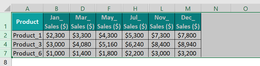
• Step 2: Right-click on a selected row number to choose Unhide in the contextual menu.
The highlighted option will unhide all the hidden rows in the chosen row range.
[Alternatively, select the required row range and press the shortcut keys Ctrl + Shift + 9 to unhide all the hidden rows in the chosen row range.]
• Step 3: Hover the cursor on column name A. Next, with the left mouse button clicked, hover the cursor on the remaining column names in the dataset to select entire columns B to M.
• Step 4: Right-click on a select column name to select Unhide in the contextual menu.
The highlighted option will unhide all the hidden columns in the chosen range.
[Alternatively, select the required column range and press the shortcut keys Alt + O + C + U or Alt + H + O + U + L to unhide all the hidden columns in the chosen range.]
We can freeze Rows and Columns in Excel using the Freeze Panes option in the View tab.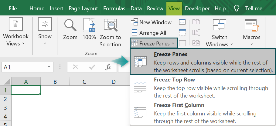
We must choose the cell where we must freeze the Rows and Columns above and on its left. And then, select the View tab → Freeze Panes option → Freeze Panes option to freeze the required Rows and Columns in the worksheet.
We can show Rows and Columns in Excel by checking the Gridlines option box in the View tab.
The above action will show the gridlines in the worksheet, forming the Rows and Columns and making the data more readable.
Use this Rows And Columns In Excel Template to follow along with the examples in this article.
Download Excel TemplateRecommended Articles
Continue with these related resources when you want the next practical step in this topic.
- Cell References in Excel
- Relative References in Excel
- Mixed References In Excel
- 3D Reference in Excel
- Structured References In Excel
Explore the full Excel Reference Functions guide or browse Excel Resources.