Column Lock In Excel

What Is Excel Column Lock?

Column lock in Excel is a feature that helps protect columns of data from unwanted editing and tampering. Also, it enables one to keep the columns seeable while scrolling to another area in the worksheet.

One can use the Excel column lock option to avoid unauthorized users adding, deleting, moving, or modifying one or multiple columns of data in a worksheet.

For example, the table below contains the sales data for ten items at different firm branches.

If the requirement is to ensure the first column containing the item codes remains visible while scrolling toward the right side of the sheet. Then, we can utilize the Freeze First Column option under the Freeze Panes feature in the View tab to lock column in Excel when scrolling.

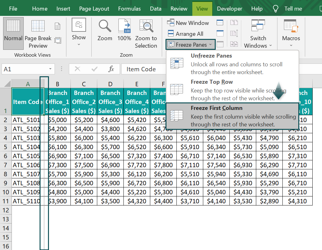
So, once we select the Freeze First Column option to lock column in Excel when scrolling, the first column, column A, freezes, indicated by the column’s bold right-side border. And column A remains visible when moving towards the last column in the dataset, while the columns scrolled in between get hidden.

What Is Excel Column Lock?

Column lock in Excel feature helps keep columns seeable while scrolling toward the last columns on the right in the dataset. And the feature helps protect data in columns from unwanted updates and changes.
Users can lock columns when they must keep certain columns seeable while scrolling across a massive dataset in a worksheet. Also, the feature is useful when they must ensure that unauthorized users do not edit or format columns of data in a worksheet.
We can lock columns in Excel using the Freeze Panes feature in the View tab and the Protect Sheet option in the Home or Review tab.

Explanation

Consider the given dataset is massive and it extends across several columns. Then, when we scroll toward the last columns in the dataset, the first few columns may not be visible after a point. And only a certain number of columns will be visible at a time for the set sheet zoom level.

In such scenarios, analyzing the entire dataset based on the columns at the beginning of the dataset can become a challenge.

Thus, the solution is to lock the columns that must be visible, even on scrolling till the last column in the dataset, using the Freeze Panes option in the View tab.

Furthermore, we may use Excel worksheets to prepare reports containing confidential data. And we may require to ensure that unauthorized parties cannot modify or edit the data, even if they have access to it.

Then, in such a case, we can lock the columns containing confidential data by password-protecting them using the Protect Sheet feature from the Home or Review tab. And only when the user knows the password can they unprotect the sheet, unlock the columns, and perform the required edits.

Excel VBA – All in One Courses Bundle (35+ Hours of Video Tutorials)

If you want to learn Excel and VBA professionally, then Excel VBA All in One Courses Bundle (35+ hours) is the perfect solution. Whether you’re a beginner or an experienced user, this bundle covers it all – from Basic Excel to Advanced Excel, Macros, Power Query, and VBA.

Start Learning Now

How to Lock Column in Excel?

We can perform column lock in Excelusing the following two methods:

Freeze Panes Feature in The View Tab
Protect Sheet Feature in The Home or Review Tab

Method #1 – Freeze Panes Feature in the View Tab

The steps to utilize the Freeze Panes feature to perform column lock in Excel from scrolling are as follows:

In the current worksheet, click the View tab → Click the Freeze Panes drop-down → Choose the Freeze First Column option to lock the first column in the worksheet.
Choosing the above option will lock or freeze the first column in the worksheet, with the column’s bold right-side border indicating the same.

On the other hand, if the requirement is to lock multiple columns. Then, here is how to achieve the desired outcome.

First, select the topmost cell in the column on the right of the last column in the set of columns we wish to lock. For example, we must lock columns A and C in a worksheet. Then, we should select cell D1.

Selecting any cell other than cell D1 in column D will freeze the rows above the selected cell. And hence, to avoid rows getting locked, we choose the topmost cell in the required column.

Click the View tab → Select the Freeze Panes drop-down → Choose Freeze Panes to lock all the columns before the chosen cell.

Furthermore, this method of column lock in Excel will keep the locked columns visible and editable while we scroll to other parts of the spreadsheet.

How to Lock Columns in Excel - Method 1 - Step 3d

Method #2 – Protect Sheet Feature in the Home or Review Tab

The steps to use the Protect Sheet feature to lock column in Excel from editing are as follows:

Select the worksheet where we need to lock columns by clicking the triangle on the top left corner of the work area. And right-click to choose Format Cells from the context menu.

How to Lock Columns in Excel - Method 2 - Step 1a

The Format Cells window opens, where we must go to the Protection tab to uncheck the Locked option. And then click OK.

Let us assume that we must lock columns B and C. Then, select columns B and C and right-click to choose Format Cells from the context menu.

The Format Cells window opens, where we must choose the Protection tab → Check the Locked option box → Click OK.

Choose the Review tab → Select the Protect Sheet option to open the Protect Sheet window.

How to Lock Columns in Excel - Method 2 - Step 3a

Otherwise, click the Home tab → Select the Format drop-down → Choose the Protect Sheet option to open the Protect Sheet window.

Enter the password in the provided field and ensure the options shown in the image below remain selected before clicking OK.

Next, another window, Confirm Password, to confirm the password will open.

Reenter the password in the Confirm Password window and click OK to close both windows.

The above steps to lock column in Excel from editing will lock the required columns B and C. And we cannot update any data or make formatting changes to the two locked columns.

On the other hand, we can update data in the remaining cells, but the formatting options will remain disabled in the worksheet.

Furthermore, the above method helps to lock column width Excel effectively. The Format Cells and Column Width options in the context menu appear greyed out on right-clicking the locked columns, ensuring we cannot change the locked columns’ width.

Examples

Check out the following illustrations for column lock in Excel to use the feature in the best possible ways.

Example #1 – Locking the First Column of Excel

The table below shows the population statistics of ten US states from 2010-22.

The above image shows the worksheet at a certain zoom level to view all the columns. And thus, the font appears small, making it difficult to read the data for analysis.

On the other hand, when the zoom level is 100%, we can view the data till column K. So, reviewing the population statistics for each state in columns beyond column K becomes challenging, as after a point, we cannot see column A, which contains the states’ names.

Thus, we can freeze column A. It will ensure we can view the state name, even when we scroll to the last column in the dataset, making data analysis more straightforward.

And the best way to achieve the desired outcome is to perform column lock in Excel using the Freeze First Column option under the Freeze Panes feature in the View tab.

Step 1: Select View → Freeze Panes → Freeze First Column in the current worksheet.

The first column in the worksheet, column A, gets locked or frozen.

Now, if we scroll towards the right of column A, column A remains visible, with the columns after column A getting hidden as we cross them. And Excel shows the column where we stop scrolling immediately after the locked column, making data analysis less cumbersome.

Furthermore, though we locked column A, it is still editable.

And thus, this method of column lock in Excel avoids the requirement of scrolling back and forth the worksheet to refer to a column in the front during data review and manipulation.

Example #2 – Lock Any Other Column of Excel

We shall see how to utilize the Freeze Panes option to lock any other column of Excel.

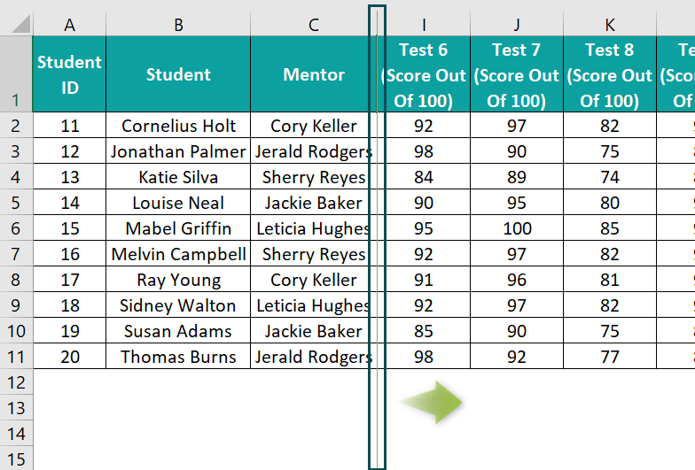
For example, the table below shows ten students’ IDs, mentors and score details.

However, scrolling the sheet to the right to view and review each student’s scores in the tests after Test 6 can be challenging. The reason is that we cannot view the student’s IDs, mentors and score details after a point.

In such scenarios, we can utilize the Freeze Panes option to perform the required column lock in Excel.

Thus, we shall lock columns till column C using the option mentioned above in this illustration. It will ensure that columns A:C, containing the students’ IDs, names, and mentors’ details, remain visible, even on scrolling till the last column in the dataset.

Step 1: To lock columns until column C, select cell D1 and click View → Freeze Panes → Freeze Panes.

Choosing the Freeze Panes option will highlight the entire column C right-side border, as shown below, indicating the frozen pane range.

And, if we scroll towards the last columns in the dataset, columns A to C remain visible, while the remaining columns get hidden as we cross them.

Thus, this option to perform column lock in Excel ensures we can view the student details while analyzing their scores in the last tests, which would not be feasible otherwise.

Example #3 – Using the Protect Sheet Feature to Lock a Column

The following table contains a list of tech companies and their stock price details. And the requirement is to ensure that unauthorized users do not edit the stock data in columns B:E.

Then, we can use the Protect Sheet feature from the Home or Review tab to perform column lock in Excel and meet our data protection requirements.

Step 1: Click the triangle on the top left corner of the work area to select the entire worksheet. And then, right-click to select Format Cells from the context menu.

The Format Cells window opens, where we must select the Protection tab.

Step 2: Uncheck the Locked option in the Protection tab in the Format Cells window. And click OK.

Step 3: Select the cell range B1:E8 (The data range to lock) and right-click to choose Format Cells from the context menu.

The Format Cells window opens, where we must select the Protection tab.

Step 4: Check the Locked option box in the Protection tab in the Format Cells window. And click OK.

Step 5: Select Home → Format → Protect Sheet to open the Protect Sheet window.

Alternatively, we can select Review → Protect Sheet to open the Protect Sheet window.

Step 6: Enter the password in the specified field for unprotecting the sheet.

Clicking OK will open the Confirm Password window.

Reenter the password, updated in the Protect Sheet window, in the Confirm Password window.

And clicking OK will password-protect the current sheet, while the other worksheets in the workbook will be available for regular use.

We can see that the Protect Sheet option in the Review tab changes to Unprotect Sheet, and all the formatting options get disabled.

Furthermore, when we try editing data in the locked or password-protected columns B:E cells, we will get the below warning message.

Also, this method helps lock column width Excel.

We can confirm the same by right-clicking the locked column range to access the Format Cells or Column Width options from the context menu, which will appear disabled.

On the other hand, the remaining cells in the worksheet will be editable, but the formatting features will be unavailable or disabled.

For example, we can select cell A7 and update the data.

However, we cannot format cell A7, as all the formatting options remain disabled.

Important Things to Note

If the requirement is to use the column lock in Excel option to lock a certain column in a worksheet. Then, select the first cell in the column on the right side of the column we must lock, and then choose the Freeze Panes option to complete the locking action.
Using the Freeze Panes feature to lock columns will ensure the locked columns remain editable.
The Protect Sheet option to lock columns ensures we cannot edit or format the password-protected columns.

Frequently Asked Questions (FAQs)

1. How do I lock an A and B column in Excel?

We can lock an A and B column in Excel using the Freeze Panes option in the View tab. This method will protect the columns from scrolling.

Let us see the steps with an example.

The table below lists employees, their designations and attendance details.

And the requirement is to lock columns A and B.

• Step 1: Select cell C1. And then, choose View → Freeze Panes → Freeze Panes.

After clicking the Freeze Panes option, the two columns get locked.

Now, if we scroll towards the last columns in the dataset, columns A and B remain visible, while the columns we cross get hidden.

Furthermore, though columns A and B get locked, they remain editable.

2. How to remove column lock in Excel?

We can remove column lock in Excel by selecting View → Freeze Panes → Unfreeze Panes.

The Unfreeze Panes option will appear under the Freeze Panes feature in the View tab when the current worksheet contains frozen columns or rows.

Otherwise, if we used the Protect Sheet option to lock columns, we must select Review → Unprotect Sheet or Home → Unprotect Sheet.

The Unprotect Sheet dialog box will open, where we must enter the password, which we used to lock columns and protect the worksheet. And then click OK to unlock the locked columns.

3. How do I lock a column but not a row in Excel?

We can lock a column but not a row in Excel by selecting the first cell in the column on the right-hand side of the column to lock and choosing View → Freeze Panes.
Otherwise, we can use the Protect Sheet option to achieve the desired outcome.

Download Template

This article must be helpful to understand the Column Lock In Excel, with its formula and examples. You can download the template here to use it instantly.

Column Lock In Excel Download

Column Lock In Excel