
What Is Compare And Match Two Columns In Excel?
Compare and Match Two Columns in Excel means that depending on the data structure, a user wants to compare the data and match them according to some conditions or scenarios to get logical results such as TRUE or FALSE.
There is no inbuilt formula to Compare and Match. However, we can use a number of functions in Excel, such as IF(), VLOOKUP(), etc., to perform the comparison and match.
For example, the image below depicts two sets of values, and we will Compare and Match two Columns in Excel by building a formula.

Select cell C2, enter the formula =A2=B2, press the “Enter” key, and drag the formula from cell C2 to C3 using the fill handle.

The output is shown above.
Key Takeaways
- Compare and Match Columns in Excel help users compare two values, check if there is a match between the same, and returns True or False if the match is found.
- Once we get the final result, we can use the Conditional formatting feature to highlight the required data or to differentiate the results from the fed output. We can apply specific formatting to cells according to certain criteria.
- Other techniques used to compare Excel columns are,
- The equals operator “=”.
- The row-by-row comparison.
- We can combine two functions, such as IF-AND, IF-OR, or use other inbuilt functions, such as VLOOKUP, EXACT, etc, to Compare and Match.
How To Compare Two Columns In Excel For Match?
We can Compare and Match data or columns in various ways, such as,
- Basic Way.
- Using inbuilt Excel functions.
Method #1 – Basic Way
The steps are:
- Type “=” equal to sign.
- Enter the first cell value or reference.
- Then, enter any operators such as =, >, <, etc.
- Enter the second cell value or reference.
- Press the “Enter” key.
Method #2 – Using Inbuilt Excel Functions
We can use,
- The inbuilt functions such as IF excel function, VLOOKUP, EXACT excel function, etc.
- Conditional formatting to highlight the compared and matched values.
Examples
We will consider some advanced scenarios to Compare and Match, namely,
- Compare Two Columns of Data.
- Case Sensitive Match.
- Change Default Result TRUE or FALSE with IF Condition.
- Highlight Matching Data.
Example #1 – Compare Two Columns of Data
The following example depicts two sets of values, and we will Compare and Match Two Columns in Excel using the formula.
In the table, the data is,
- Column A contains Value 1.
- Here, column B contains Value 2.
- Column C contains the Match Output.

The steps to Compare and Match Two Columns are as follows:
- 1: Select cell C2, and enter the formula =A2=B2.

- 2: Press the “Enter” key. The result is “TRUE”, as shown below.

- 3: Drag the formula from cell C2 to C9 using the excel fill handle. The output is shown below.

[Note: Further, we can use conditional formatting too. The cells that are not matched are highlighted in yellow color, and cells C3 and C6 are not matched, as shown in the below image.]

Example #2 – Case Sensitive Match
The following example depicts two sets of values, and we will Compare and Match Two Columns to the Case Sensitive Match using the EXACT formula.
In the table, the data is,
- Column A contains Value 1.
- Here, column B contains Value 2.
- Column C contains the Match Output.

The steps to Compare and Match Two Columns using the Exact() function are as follows:
- 1: Select cell C2, and enter the formula =EXACT(A2,

- 2: Select the cell that contains text 2, i.e., “B2”, and close the brackets. Now, the complete formula is =EXACT(A2, B2)

- 3: Press the “Enter” key. The result is “TRUE”, as shown below.

- 4: Drag the formula from cell C2 to C9 using the fill handle. The output is shown below.

[Note: Further, we can use conditional formatting too. The cells that are not matched are highlighted in green color, and cells C3, C7, and C9 are not matched, as shown in the below image.]

Example #3 – Change Default Result TRUE or FALSE with IF Condition
The following example depicts two sets of string values, and we will Change the Default Result to TRUE or FALSE using the IF excel formula.
In the table, the data is,
- Column A contains String 1.
- Here, column B contains String 2.
- Column C contains the Match Output.

The steps to Compare and Match Two Columns using the IF() formula are as follows:
- 1: Select cell C2, and enter the formula =IF(A2=B2,
[Note: Select the cell that contains logical test condition, i.e., “A2=B2.”]

- 2: Select the cell that contains a value if true, i.e., “Matched String”.

- 3: Select the cell that contains a value if false, i.e., “Unmatched String”, and close the brackets. The complete formula is =IF(A2=B2, “Matched String,” “Unmatched String”).

- 4: Press the “Enter” key. The result is “Unmatched String”, as shown below.

- 5: Drag the formula from cell C2 to C5 using the fill handle. The output is shown below.

[Note: The cells that are not matched are highlighted with yellow color using conditional formatting. Cells C2 and C4 are not matched, as shown in the below image.]

Example #4 – Highlight Matching Data
The following example depicts two sets of values, and we will Compare and Match Two Columns and Highlight Matching Data.
In the table, the data is,
- Column A contains Value 1.
- Column B contains Value 2.

The steps to Compare and Match Two Columns and highlight the result are as follows:
- 1: First, select the cells containing the values, i.e., A2:B6. Then, select the “Home” tab → go to the “Styles” group → click the “Conditional Formatting” option drop-down → select the “New Rule…” option, as shown below.

- 2: The “New Formatting Rule” window pops up.
- Select the “Use a formula to determine which cells to format” option from the “Select the Rule Type:” list.
- Enter the formula “=$A2=$B2” in the “Edit the Rule Description:”.
- Select the “Format” button.

- 3: The “Format Cells” window pops up.
- Select the color from the Fill option from the menu, here, Blue color.
- Click OK in the “Format Cells” window.

- 4: Click OK in the “New Formatting Rule” window.

- 5: The matched cells are highlighted as shown in the below image.

Important Things To Note
- Compare and Match columns in Excel to check each cell against the other cells to identify a match.
- If the match is missing, then the relevant message is returned.
- Compare and Match columns in Excel can be done by highlighting each column’s unique or duplicate values.
- Conditional Formatting is used to display unique or duplicate cells or columns.
Frequently Asked Questions (FAQs)
Excel uses data for storage, manipulation, and decision-making that helps convey information to the user. Data analysis tools gather the information used in marketing and sales decisions. The formula does not contain information. Some datasets are huge and linked to each other. A data analyst needs to compare two columns across the same or different spreadsheets, and doing it manually is a tedious task. It takes a huge amount of time to find the missing data.
Comparing two columns in Excel finds out whether the cell contains matched data. It displays as output TRUE or FALSE, for Match or Not Match, or any other message defined by the user.
The following example depicts two sets of values, and we will Compare and Match Two Columns in Excel to using VLOOKUP Excel formula.
In the table, the data is,
• Column A contains Value 1.
• Column D contains Value 2.
• Column E contains the Match Output.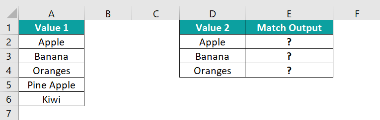
The steps to Compare and Match using VLOOKUP() are as follows:
• 1: Select cell E2, and enter the formula =VLOOKUP(A2, D2:D4, 1, TRUE)
[Note: The arguments are, the cell that contains a lookup value, i.e., “A2”, the cell that contains a table array, i.e., “D2:D4”, the cell that contains a column index number, i.e., “1”, and the cell that contains a range lookup, i.e., “TRUE”.]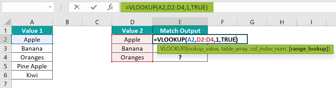
• 2: Press the “Enter” key. The result is “Apple”, as shown below.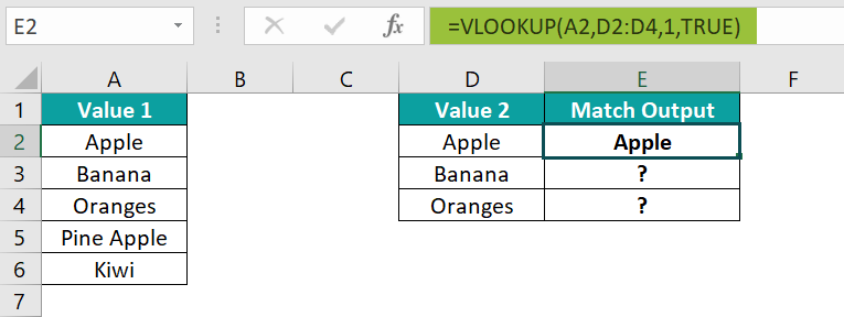
• 3: Drag the formula from cell E2 to E4 using the fill handle. The output is shown below.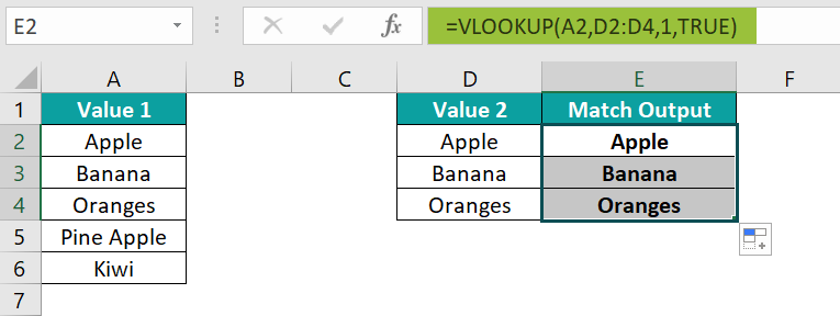
The other methods used to Compare two Columns in Excel are by using AND and OR functions along with the IF function.
• To find matches in all cells within the same row in the table of the same values, the IF-AND formula is =IF(AND(A2=B2, A2=C2), “Full match,” “No match”).
• To find matches if any two cells are in the same row, the IF-OR formula is =IF(OR(A2=B2, B2=C2, A2=C2), “Match,” “No match”).
Download Template
This article must help understand the Compare and Match Columns in Excel formula and examples. You can download the template here to use it instantly.