
What Are Errors In VLOOKUP?
We can fix VLOOKUP errors in simple steps. The VLOOKUP errors in Excel occur when one does not follow the VLOOKUP() syntax and rules diligently and also due to the function’s limitations. The common errors in VLOOKUP are #N/A, #VALUE!, #REF, and #NAME.
Users can identify the root causes for the specific VLOOKUP error, such as typo mistakes in the function argument values, and apply the corrective measures.
Use this Fixing VLOOKUP Errors Template to follow along with the examples in this article.
Download Excel TemplateFor example, the first table lists fruits and their quantities.
And suppose the requirement is to find the quantity of the fruit specified in the second table by fetching the required data from the first table using the VLOOKUP() in the target cell G2.
However, the result shows one of the common VLOOKUP errors, #N/A, in the target cell.

The reason for such common VLOOKUP errors is that the function fails to find the referenced value.
In the above example, when the VLOOKUP() tries looking up the fruit Orange in the first table, it does not find the value in the source data. And hence, it returns the #N/A error.
We can fix such VLOOKUP errors by ensuring the first column in the source table includes all the lookup values.
Otherwise, we can apply the VLOOKUP() within the IFERROR() to display a customized text instead of the error value.

Key Takeaways
- VLOOKUP errors result from not applying the function syntax properly and the function’s limitations and we can fix them easily.
- Ensure the lookup_value does not contain additional spaces and typo errors and the numeric values’ data format in the table_array is not text. Also, the lookup_value should appear in the first column in the table_array and must not be below the smallest value in the column. These measures will avoid the #N/A error.
- Similarly, we should ensure the col_index_num is not less than 1, and the lookup_value length does not exceed 255 characters to avoid the #VALUE error.
- The col_index_num should not exceed the total number of columns in the table_array, and the function name should be correct. Otherwise, the VLOOKUP() will return the #REF and #NAME errors.
Top 4 Errors In VLOOKUP And How To Fix Them?
We shall understand the VLOOKUP errors and solutions to eliminate them and achieve the desired VLOOKUP function output.
#1 – Fixing #N/A Error In VLOOKUP
The #N/A VLOOKUP errors occur due to the following reasons:
- Additional spaces in the lookup_value.
- Typo error in the lookup_value.
- The data format of numeric value in the table_array is Text.
- The lookup_value does not occur in the first column of the table_array.
- The lookup_value is below the smallest value in the table_array’s first column.
For example, the first table contains the source data, with which we must update the second and third tables using the VLOOKUP() in cell range H2:H4 and H7:H8.
However, on applying the function in the target cells, we obtain the VLOOKUP errors, as shown below.

Here is how to fix the #N/A VLOOKUP errors.
Solution
- Step 1: The VLOOKUP() returns the #N/A error in cell H2 because the lookup_value in cell G2 contains trailing spaces.
Thus, we shall modify the VLOOKUP() formula by introducing the TRIM() to remove the trailing spaces from the lookup value. And for that, we must select cell H2, enter the following formula, and press Enter.
=VLOOKUP(TRIM(G2),B1:E11,4,0)

The TRIM() deletes the additional spaces following the specified lookup value in cell G2. And then, the VLOOKUP() searches for the employee name specified in cell G2 of the second table in the first table. And as we supply the col_index_num as 4, the function returns Kendra Bowman’s designation, Specialist.
- Step 2: Though we supplied the lookup_value directly as a text in the VLOOKUP() in cell H3, the employee name is incorrect. So, the supplied lookup_value contains a typo error, which leads to the function returning the #N/A error. And it is a scenario of VLOOKUP errors with text.
Thus, to fix it, select cell H3, enter the VLOOKUP() as shown below, and press Enter.
=VLOOKUP(“Percy Norton”,B1:E11,4,0)

Once we supply the employee name with the correct spelling, the #N/A error in cell H3 gets eliminated.
- Step 3: The lookup_value supplied in the VLOOKUP() in cell H4, Allen Reed, is not present in the first table, leading to the function returning the #N/A error.
In such a case, we can use the IFERROR() to show a customized text instead of the error value. Thus, we can select cell H4, enter the VLOOKUP() within the IFERROR(), and press Enter.
=IFERROR(VLOOKUP(G4,B1:E11,4,0),”Data Not Available”)

The VLOOKUP() output remains the same, #N/A error. But the IFERROR() displays the specified text “Data Not Available” instead of the error value.
Next, cells H7:H8 show the scenarios of VLOOKUP errors with numbers.
- Step 4: Though the source table contains the specified lookup_value, 1300, the data format of the value is Text. And thus, it results in the VLOOKUP() returning the #N/A error in the target cell H7.

In such a case of VLOOKUP errors with numbers, we must correct the data format of the numeric value to overcome the error.
Thus, in the above example, we must select the source table cell D9, containing the lookup value. And then, click the error warning icon to pick the second option for converting the value into a number.

On clicking the option highlighted in the above image, the error in cell H7 gets fixed, and we obtain the required designation.

- Step 5: The cell H8 formula shows that the VLOOKUP() performs an approximate match. However, as the specified lookup value in cell G8 in the third table is below the smallest value in column D of the source table, the function returns the #N/A error.
On the other hand, if column D did not have the values sorted in ascending order, it would also lead to the function returning the #N/A error.
Thus, we can use the IFERROR(), as explained in step 3, to show a customized text in place of the error value. And for that, we must select cell H8, enter the following formula containing the VLOOKUP() within the IFERROR(), and press Enter.
=IFERROR(VLOOKUP(G8,D1:E11,2,1),”Data Out Of Range”)

#2 – Fixing #VALUE! Error In VLOOKUP
The #VALUE! VLOOKUP error occurs due to the following reasons:
- Missing mandatory arguments.
- The col_index_num argument is less than 1.
- The lookup_value argument value length exceeds the maximum characters of 255.
For example, the first table contains product codes and prices. And we use this source data to update the prices in column G of the second table using the VLOOKUP() in the target cells.
However, on applying the function in the target cell range G2:G4, we see the VLOOKUP errors, as shown below.

Here is how to fix the #VALUE! VLOOKUP errors.
Solution
- Step 1: The VLOOKUP() in cell G2 has the lookup_value argument missing. So, the function does not have the value to search in the source table for fetching the required data. Also, the arguments’ order is incorrect, leading to the function returning the #VALUE! error.
Thus, select cell G2, enter the below VLOOKUP(), which includes all three mandatory arguments and one optional argument, and press Enter to fix the error.
=VLOOKUP(F2,C1:D8,2,0)

- Step 2: The VLOOKUP() looks up the value from left to right. So, the col_index_num argument value in the VLOOKUP() should be positive.
But in this case, the col_index_num argument value in the VLOOKUP() in cell G3 is below 1, -2. And a negative col_index_num indicates looking up in the reverse direction, which leads to the function returning the error.
Thus, select cell G3, enter the VLOOKUP() with the required positive col_index_num argument value, and press Enter.
=VLOOKUP(F3,C1:D8,2,0)

- Step 3: Sometimes, the lookup_value might exceed 255 characters. Then, in such scenarios, we may see the VLOOKUP error.
In this example, cells C7 and F4 contain data with over 255 characters.

We can resolve the issue by reducing the number of characters and ensuring the lookup_value argument value includes below 255 characters.
Thus, we will select the junk data from cells C7 and F4.


And delete the selected data in the two cells, one at a time.

Finally, press Enter or click anywhere in the sheet to obtain the correct data in the target cell.

Suppose the lookup_value had below 255 characters, but the source table contained a value with over 255 characters instead of the lookup value. Then, it would be a case of the #N/A VLOOKUP errors with text, as seen in the previous section.
#3 – Fixing VLOOKUP #REF Error
The #REF VLOOKUP error occurs when we supply the col_index_num argument value, which exceeds the total columns in the table_array.
For example, the first table contains a list of US states and their capitals and population figures for 2022.
The requirement is to update the state’s population mentioned in the second table based on the first table data. Assuming the target cell is I2.
So, we select the target cell and apply the VLOOKUP() to achieve the required data, as shown below. However, the VLOOKUP() returns the #REF! error in cell I2.

The #REF VLOOKUP error is because the entered col_index_num argument value is 4, a value more than the total columns in the source table, 3.
So, here is how to fix such #REF VLOOKUP errors.
Solution
- Step 1: Select cell I2, enter the VLOOKUP(), and press Enter.
=VLOOKUP(H2,D1:F7,3,0)

On the other hand, suppose we enter a col_index_num lower than the total columns in the table_array. Then, the result will be the corresponding value from the column, which is at the position indicated by col_index_num from the leftmost column, instead of an error value.
For example, in the above example, we require the population of Texas. So, col_index_num is 3. Had we supplied the argument as 2, the function would return Austin instead of an error value, though it is incorrect.
#4 – Fixing VLOOKUP #NAME Error
The #NAME VLOOKUP error occurs when the entered function name is incorrect.
For example, the first table lists books and their authors.
Suppose the requirement is to update the author name in cell H2 for the book specified in the second table based on the first table data. Then, we will apply the VLOOKUP() in the target cell to obtain the required author name.
However, the output in the target cell is the #NAME? error.

The error is because we entered the incorrect function name, BLOOKUP, instead of VLOOKUP.
And here is how to fix the #NAME VLOOKUP errors.
Solution
- Step 1: Select cell H2, enter the VLOOKUP() as shown below, and press Enter.
=VLOOKUP(G2,D1:E7,2,0)

#5 – VLOOKUP Not Working Between Two Sheets
The VLOOKUP errors we saw in the above sections can occur when we look up values from other sheets due to the reasons discussed previously.
However, it is possible to get VLOOKUP errors due to other reasons when applying the function between multiple sheets.
Let us see the common scenarios when we can encounter VLOOKUP errors and solutions to fix the issues.
- External Reference to Another Worksheet or A Workbook Is Incorrect
Providing an incorrect external reference to another worksheet in the same or another workbook leads to VLOOKUP errors, such as the #N/A.
For example, the first workbook contains a sheet showing the prices of three stocks in Jan and Feb.
And suppose another workbook contains the prices of the three stocks in Mar, which we must use to update the March month data in the first workbook. Assume the target cell range are F2:F4 in the first workbook.


Then, we will first apply the VLOOKUP() in the target cell F2, using the external reference to the other worksheet in the second workbook.

However, when we press Enter, the window shown in the below image appears, asking us to update the source value.

And if we choose to skip the update and close the window, we see the #N/A error as the VLOOKUP() output in the target cell F2.

The reason is that the second workbook’s name is incorrect in the reference specified in the VLOOKUP().
So, here is how to overcome such VLOOKUP errors.
Solution
- Step 1: Select the target cell F2, enter the VLOOKUP() with the correct external reference to the worksheet in the second workbook, and press Enter.
=VLOOKUP(C2,'[Mar Stock Price Data.xlsx]Mar_Stock_Prices’!$D$1:$E$4,2,0)

- Step 2: Implement the formula in cell range F3:F4 using the fill handle.

- The Full Path to The Closed Workbook Referenced In VLOOKUP() Is Incorrect
Continuing the previous example, suppose the second workbook is closed. And we provide the full path as the external reference to the closed file in the VLOOKUP() in the target cell F2 of the first workbook, as shown below.

Then, pressing Enter opens the window to update the source value.

And if we close the window, the VLOOKUP() returns the #N/A error in the target cell F2.

The reason is that the specified full path to the closed file in the formula is incorrect.
Solution
Here is how to fix the VLOOKUP error.
- Step 1: Select cell F2, enter the VLOOKUP() with the correct full path to the closed workbook containing the source data, and press Enter.
=VLOOKUP(C2,’C:\Users\Downloads\Excel Mojo\Excel files copy\Fixing VLOOKUP Errors_Worksheets[Mar Stock Price Data.xlsx]Mar_Stock_Prices’!$D$1:$E$4,2,0)

- Step 2: Using the fill handle, update the formula in cell range F3:F4.

- Worksheets Are Open in Separate Instances of Excel
Suppose we have two workbooks, Carla Hunter Scores and Mathematics Scores. And we open them in different instances.
- Step 1: Right-click the Excel icon pinned in the Taskbar.

And then, pressing the Alt key, left-click the Excel icon in the Taskbar. Continue pressing the Alt key till the below message box opens.

- Step 2: Click Yes to open a new instance of Excel.

The above action will open the Excel software, from where we will open the first workbook, Carla Hunter Scores, by clicking the file name in the above-shown window.

- Step 3: Next, we will open the second workbook in another instance of Excel, following the abovementioned steps.

Suppose the requirement is to update the Mathematics score of Carla Hunter in cell C3 in the Carla Hunter Scores workbook based on the Mathematics Scores workbook data. Then, using the VLOOKUP() in the target cell will fetch us the required data.
- Step 4: Select cell C3 and type the VLOOKUP(), as shown below.
=VLOOKUP(A3,

Next, when we go to the second workbook to update the table_array argument in the VLOOKUP(), Excel does not show the required range in the formula.

The reason is that we opened the two workbooks in separate instances of Excel. And we can confirm the same by right-clicking the Taskbar and picking Task Manager from the menu to open the Task Manager window. Otherwise, we can use the keyboard shortcut Ctrl + Shift + Esc to access the Task Manager window.

The Task Manager window shows two instances of Excel, which causes the VLOOKUP function not to work.

Here is how to fix such VLOOKUP errors.
Solution
- Step 5: Close the two workbooks and reopen them in the same Excel instance. And we can do so by opening the two files one by one from their respective locations.
Furthermore, we can confirm by checking the Task Manager, which will show one Excel instance.

- Step 6: Select cell C3 in the Carla Hunter Scores workbook, and enter the VLOOKUP(), as shown below.
=VLOOKUP(A3,

Next, go to the second workbook. Excel will show the VLOOKUP() formula that we started entering in cell C3 in the Carla Hunter Scores workbook in the second workbook’s Formula Bar.

Update the table_array argument and complete the VLOOKUP() formula as shown below.
=VLOOKUP(A3,'[Mathematics Scores.xlsx]Mathematics_Scores’!$A$1:$B$6,2,0)

And pressing Enter will execute the VLOOKUP() in the target cell C3 in the Carla Hunter_Scores workbook.

Important Things To Note
- Supply all mandatory arguments’ values to the VLOOKUP(). Otherwise, it may lead to VLOOKUP errors.
- When using the VLOOKUP() with more than one workbook involved, ensure the provided file path or the external reference to the source workbook is accurate. Also, open the files in the same instance to avoid the VLOOKUP function not working.
Frequently Asked Questions (FAQs)
The correct syntax for VLOOKUP function is as follows: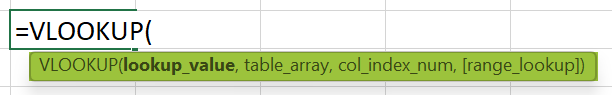
where,
• lookup_value: The value we require to look up.
• table_array: The cell range in which the function should search for the lookup_value and the return value.
• col_index_num: The column from the leftmost column in the source table containing the return value.
• range_lookup: It indicates whether the VLOOKUP() must find the approximate or an exact match. A value of 1 interprets as an approximate match, and 0 indicates an exact match.
And while the first three arguments are mandatory, the last argument is optional.
The causes of VLOOKUP errors are as follows:
• The VLOOKUP function is case-insensitive.
• Inserting or deleting a column from the source table.
• Copying a VLOOKUP() formula from one cell into another may change the cell references.
We can overcome the 255-character limit in VLOOKUP using the INDEX and MATCH functions.
For example, the first table contains a list of item codes and batch details.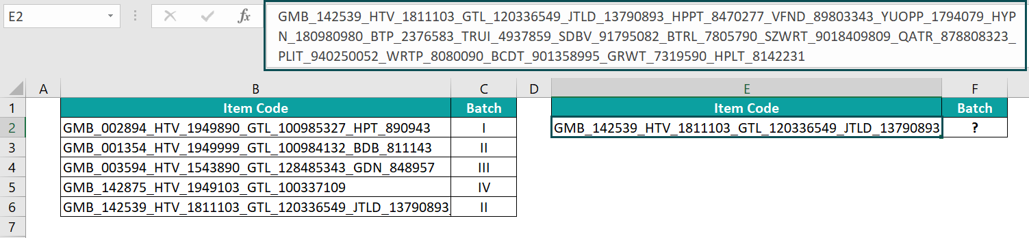
Suppose the requirement is to obtain the batch detail of one of the item codes specified in the second table based on the data in the first table. And assume the target cell is F2.
Then, in such a scenario, we will select the target cell F2, apply the VLOOKUP(), and press Enter, as shown below.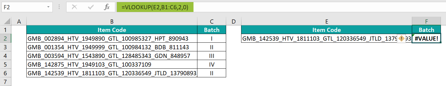
However, the VLOOKUP() returns the #VALUE! error because the lookup_value contains more than 255 characters.
Thus, we can use the INDEX and MATCH functions to overcome the issue, as explained below:
• Step 1: Select the target cell F2 and enter the formula containing the INDEX and MATCH functions.
=INDEX(C2:C6,MATCH(TRUE,INDEX(B2:B6=E2,0),0))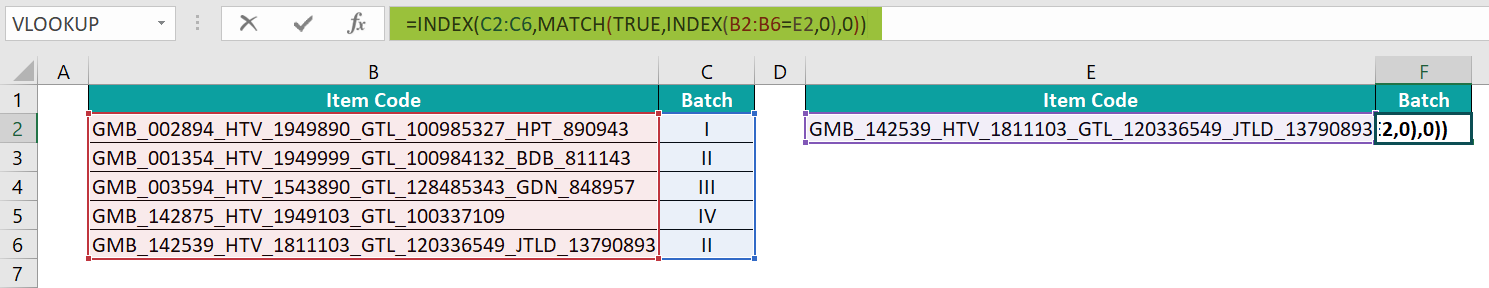
• Step 2: Press Ctrl + Shift + Enter to execute the expression as an array formula.
{=INDEX(C2:C6,MATCH(TRUE,INDEX(B2:B6=E2,0),0))}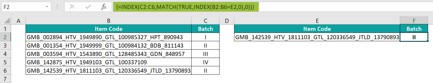
The term B2:B6=E2 in the inner INDEX() gives an array of TRUEs and FALSEs, {FALSE;FALSE;FALSE;FALSE;TRUE}. Next, MATCH() finds the match for TRUE in the fifth element in the array. So, it returns the value 5 as the output.
And then, the INDEX() returns the value in the fifth cell in the cell range C2:C6, II as the required batch.
Use this Fixing VLOOKUP Errors Template to follow along with the examples in this article.
Download Excel TemplateRecommended Articles
Continue with these related resources when you want the next practical step in this topic.
- Errors In Excel
- Excel Troubleshooting
- Excel Formula Not Working
- Circular Reference in Excel
- IFERROR In Excel
Explore the full Excel Errors and Troubleshooting guide or browse Excel Resources.