VLOOKUP From Another Sheet

What Is VLOOKUP From Another Worksheet?

The VLOOKUP function in Excel retrieves the required data from the dataset based on the lookup_value within the same sheet. VLOOKUP From Another Worksheet helps us work on scenarios where we may have to retrieve the information from a different worksheet or workbook.

What Is VLOOKUP From Another Worksheet?

The VLOOKUP function can fetch the data from different worksheets and different workbooks.
When we fetch the data from different worksheets of the same workbook using the named range, we can use the table_array.
When we apply the VLOOKUP function from different worksheets, we will get the worksheet name along with the table_array range.
When we apply the VLOOKUP from different workbooks, we will get the workbook name and worksheet name along with the table_array range.

How To Use VLOOKUP From Another Worksheet (Same Workbook)?

When the main table or lookup table is in a different worksheet of the same workbook, the VLOOKUP application is similar to what we usually apply in the same worksheet.

The only difference between working with the same worksheet and a different worksheet is that we need to switch to the different worksheets to select the table_array for the VLOOKUP function. However, when we switch, we will face many challenges.

Excel VBA – All in One Courses Bundle (35+ Hours of Video Tutorials)

If you want to learn Excel and VBA professionally, then Excel VBA All in One Courses Bundle (35+ hours) is the perfect solution. Whether you’re a beginner or an experienced user, this bundle covers it all – from Basic Excel to Advanced Excel, Macros, Power Query, and VBA.

Start Learning Now

Example #1 – VLOOKUP from Another Worksheet with Manual Selection of the Table-array

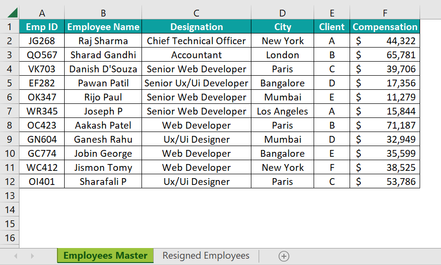
Consider the following data in Excel. The “Employee Master” worksheet, contains the employee list and all the other necessary information.

VLOOKUP From Another Worksheet - Example 1

The “Resigned Employees” worksheet has the following information.

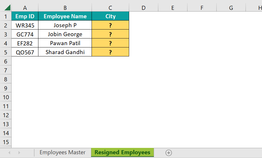
VLOOKUP From Another Worksheet - Example 1 - 1

This worksheet contains the list of employees who have resigned in the current month and need to identify the “City” they belong to from the first worksheet, “Employee Master”.

The steps to use the VLOOKUP function are,

Step 1: In the “Resigned Employees” worksheet, enter the VLOOKUP function in cell C2.

Step 2: Choose the lookup_value as cell A2.

Step 3: We must choose the table_array from the “Employee Worksheet”. Switch to the “Employee Master” worksheet first.

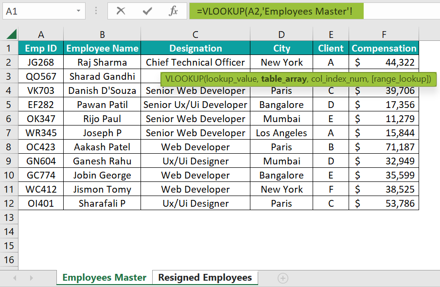
Step 4: Choose the table_array from A2:F12.

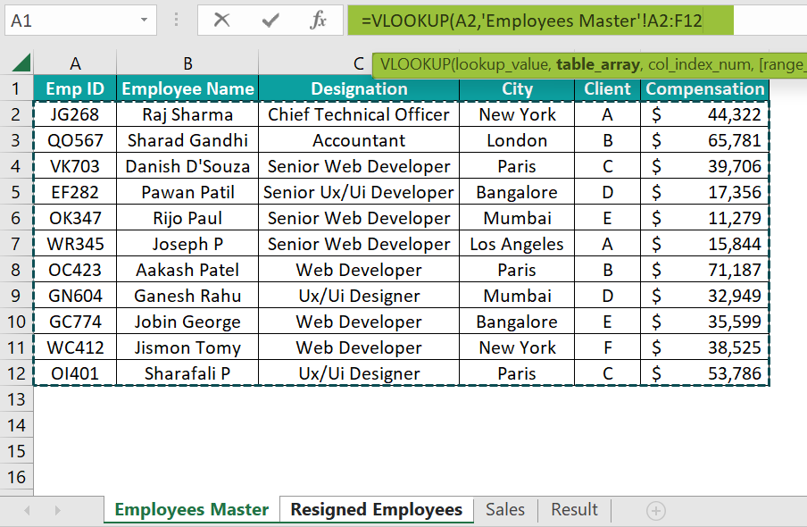
Step 5: Since we need to apply the same formula to different employees, make the table_array selection absolute, by pressing the F4 key once, and the dollar symbols get inserted.

Step 6: Do not switch to the “Resigned Employees” worksheet. Stay in the table_array selection sheet, and enter the column index number as 4 to get the city information from the 4^th column of the table_array selection.

Step 7: Enter the range lookup as FALSE or 0 to get the exact match.

Step 8: Close the bracket and press the “Enter” key to get the city name for the first resigned employee.

Immediately, we are back to the “Resigned Employees” worksheet with the VLOOKUP retrieving the city name for the first resigned employee. Drag the formula from cell C2 to C5 using the fill handle.

Now we have got the city name for all the resigned employees.

[Special Note: Difference Between the Same Worksheet and Another Worksheet Reference

Now let us understand the difference between the reference given by the same worksheet and a different worksheet.

Take a look at the following image.

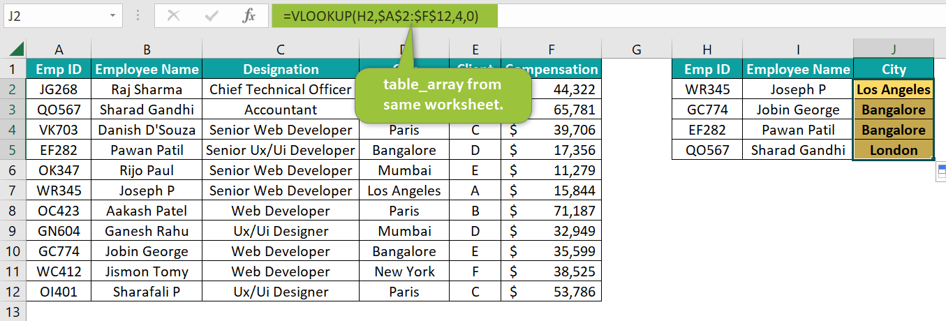
The only difference in the above two images is the table_array argument of the VLOOKUP function. So, when we get the table_array reference from the different worksheets, we have the worksheet name we are referring to in single quotes followed by an exclamation mark (!).

This shows the location of the table_array.

Example #2 – VLOOKUP from Another Worksheet with Named Ranges

Continuing with #Example 1, we will see the dynamic way of selecting the table_array range from the same sheet.

Create a Named Range for the Table_array

Using the named range, we can easily select the table_array from any worksheet within the same workbook.

The steps to create a named range are,

Step 1: Go to the table_array worksheet “Employee Master”, and select the range from A2:F12.

VLOOKUP From Another Worksheet - Example 2 - Step 1

Step 2: Select the “DataRange” option from the drop-down in the name box.

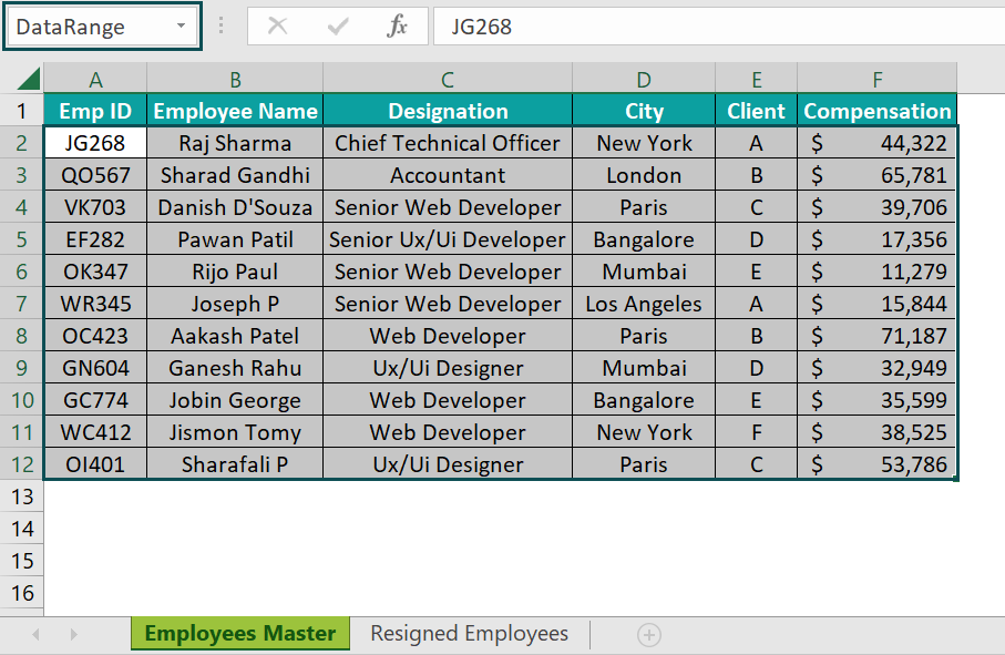
Now, we can refer to the range A2:F12 from the worksheet “Employee Master” by entering the name “DataRange”.

To test the working of the named range, select any empty cell in the worksheet “Employee Master”, enter an equal sign, and start entering the given name.

The moment we enter the name, Excel’s IntelliSense list shows the matching result for the same.

Choose the name “DataRange”. It immediately highlights the range, A2:F11, in the blue rectangular selection of the data range, as shown below.

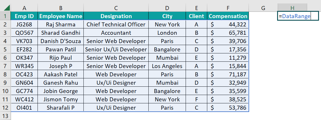
The steps to reference the range A2:F11 using the VLOOKUP function are,

Step 1: In the “Resigned Employee” worksheet, enter the VLOOKUP function.

VLOOKUP From Another Worksheet - Using Named Range - Step 1

Step 2: Choose the lookup_value as cell A2.

Step 3: We will give the table_array reference, which is in a different worksheet, i.e., the “Employee Master” worksheet. However, instead of going to that worksheet to select the table_array range, enter the name, i.e., “DataRange”.

Step 4: Enter the column index number as 4 (depending on which column information we are retrieving) and range lookup as 0 to get the exact matching result.

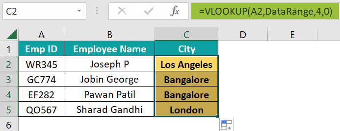
We get the result, same as the previous example, using the named range, without moving to other worksheets to select the table_array.

How To Use VLOOKUP From Another Worksheet (Different Workbook)?

We will apply VLOOKUP from a different workbook using the same data in the earlier examples, but this time in two different workbooks.

Example #1

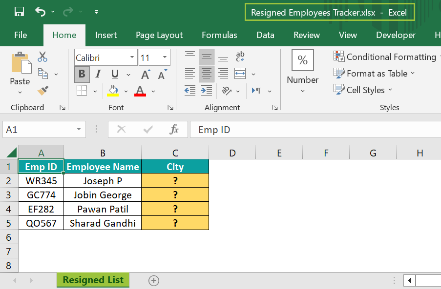
In the workbook “Resigned Employees Tracker”, we have the following resigned employees list.

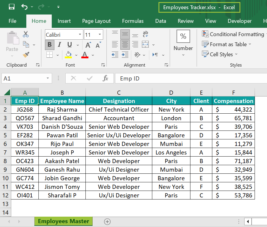
In the workbook “Employees Tracker”, we have the data of employee’s master like the following.

VLOOKUP From Another Worksheet - Different Workbook - Example 1 - 2

The steps to retrieve the city information from the “Employee Tracker” workbook to the “Resigned Employees Tracker” workbook, are as follows:

Step 1: In the “Resigned Employees Tracker” workbook, enter the VLOOKUP function and choose the lookup_value as cell A2, i.e., EMP ID.

Step 2: To choose the table_array from a different workbook, go to the “Employees Tracker” workbook. When we navigate to different workbooks, the VLOOKUP function is still active in the formula bar, as shown below.

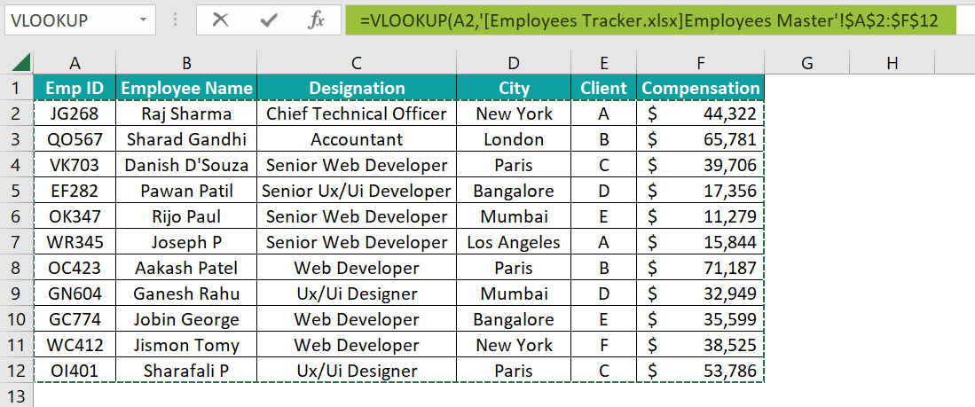
Step 3: Choose the table range from A2:F11. When we select the table_array, we see a lengthy argument inserted, and the selected range becomes an absolute reference (dollar sign) automatically.

Step 4: Enter the column index number and range lookup as 4 and 0, respectively.

Step 5: Close the bracket and press the “Enter” key to get the result.

We are back to the “Resigned Employees Tracker” workbook, and we can see the city name results.

[Note: Some of the important tips to remember are,

Table_array Break UP

‘[Employees Tracker.xlsx]Employees Master’! $A$2:$F$12

In the above syntax, the first part, which is in brackets ([ ]) ‘[Employees Tracker.xlsx] is the workbook name, and the text following after the brackets ([ ]) Employees Master’, is the worksheet name in that workbook.

Then the range of cells $A$2:$F$12 is selected in that worksheet.

What is the Table_array When We Close the Workbook?

The source workbook “Employees Tracker” is open, so in the formula, we see only the workbook name and worksheet name.

However, when we close the source workbook “Employees Tracker”, this is not the case.

Different Workbook - Example 1 - Step 5a

We can see an even bigger value. The texts appearing before the workbook name is the folder path to the source workbook saved.

‘C:\Users\Jeevan\Downloads\Excel Mojo\Excel files copy\

This is the folder path in which we have saved our workbook “Employees Tracker”.]

Example #2 – Deal with Error Values from Different Workbooks

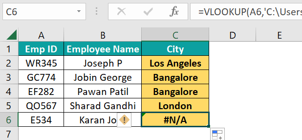
If the lookup_value does not find in the source table_array, we will get the #N/A error.

For instance, look at the following image. At the end, we have added a new employee id that is not there in the source file, so we get the #N/A error.

VLOOKUP From Another Worksheet - Different Workbook - Example 2

To deal with these errors, we can use the IFERROR function.

VLOOKUP From Another Worksheet - Different Workbook - Example 2 - 1

Here, the IFERROR excel function checks for any error value, and returns the text “Not Available” instead of the #N/A error.

Important Things To Note

The named range makes the selected data range an absolute reference, so there is no need to use the F4 key.
Whenever we select the table_array from different workbooks, the range selection becomes an absolute reference by default.
If we use the named range for the table_array and if that named range is deleted, then we will get the #NAME? error.
Whenever we apply the VLOOKUP from another workbook, always use paste special to retain only the value because if we delete the source workbook, we will lose the data in the formula sheet.

Frequently Asked Questions (FAQs)

1. How to VLOOKUP from another sheet with multiple columns?

To VLOOKUP from another sheet for multiple columns, first, we need to lock the table_array range by pressing the F4 key once. Once we get the value for one column, then change only the column index numbers accordingly.

2. Why is my VLOOKUP not working between sheets?

VLOOKUP should work for different sheets, however, if we are getting the #N/A error, then the lookup_value is not available in the table_array that we have specified.
We get the #REF error because after the VLOOKUP is applied, the table_array must have been deleted, or the column index number provided is not within the range of the table_array.

3. How to VLOOKUP from another sheet with multiple criteria?

To VLOOKUP from another sheet with multiple criteria values, we must first concatenate the multiple criteria columns in the table_array sheet.

For instance, look at the following data in the Sales worksheet.

And in the Result sheet, we have the criteria set up like the following.

In cell A2, we have a drop-down list to select the salesperson, and in cell B2, a drop-down list of regions.

So, whenever users select the salesperson and region combination, our VLOOKUP will return the sales value for the selected salesperson and region.

To do this, first, we need to create a concatenation column in the source worksheet.

Then in the VLOOKUP formula, while selecting the lookup_value, choose both salesperson and region.

Choose the table_array in the source worksheet starting from the helper column.

Mention the column index number and range lookup as per the requirement, and we should see the result.

Now whenever users change the drop-down list values accordingly, the VLOOKUP function retrieves the selected combination result.

Download Template

This article must help understand VLOOKUP from Another Worksheet with its formulas and examples. You can download the template here to use it instantly.

VLOOKUP From Another Sheet Download

Employees Tracker Download

Resigned Employees Tracker Download