TOROW in Google Sheets

What is TOROW in Google Sheets?

The TOROW function in Google Sheets converts a range or array into a single row by stacking values horizontally. In simpler words, it helps flatten the multi-column or tabular data into one continuous row. This is useful when you want to combine data from multiple rows into a single horizontal list for presentation, JOIN, or formulas that require a row input.

Unlike manual copy-and-paste, TOROW handles entire arrays dynamically and can ignore blanks or errors if needed. For example, given a dataset in A1:C3, you can flatten it into one row with:

=TOROW(A1:C3)

The function reads the range (by default) row by row and outputs a single row array that contains all values in sequence.

Syntax

=TOROW(array_or_range, [ignore], [scan_by_row])

Parameters:

1. array_or_range → The input data range or array you want to convert into a single row.
2. ignore (optional) → Controls what to exclude from the output:
   • 0 → Include all values (default).
   • 1 → Ignore blanks.
   • 2 → Ignore errors.
   • 3 → Ignore blanks and errors.
3. scan_by_row (optional) → Defines the direction of stacking:
   • TRUE → Stack by row (default).
   • FALSE → Stack by column.

How To Use TOROW Function in Google Sheets?

The TOROW function is perfect when you need a single horizontal list created from a wider table. Let us look at a simple example. TOROW can be used by either by typing it manually or via the Google Sheets menu.

Entering TOROW Manually

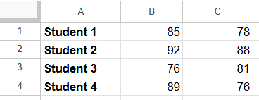
Step 1: Prepare the data and enter it in a Google Sheet. This sample table shows values spread across three columns.

Step 2: Click an empty cell where you want the flattened row to appear like A5. Type the TOROW formula:

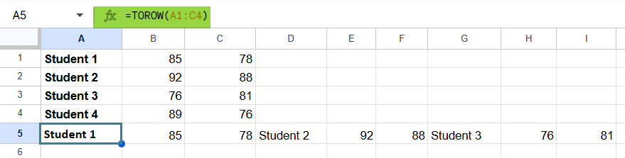
=TOROW(A1:C4)

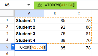
Here, A1:C4 is the data range you are converting.

Step 3: Press Enter. Google Sheets will display the combined row array.

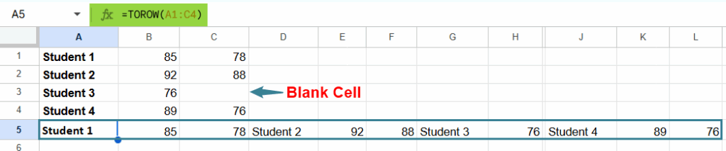
 If the range contains blanks and you want to skip them, use:

=TOROW(A1:C4, 1)

Insert Through Google Menu Bar

1. Go to Insert → Function → Array → TOROW.
2. Select the array_or_range you want to flatten.
3. Optionally set the ignore and scan_by_row parameters in the function helper.
4. Press Enter to produce the single row output.

Examples

In many real-life scenarios, we need to organize or summarize data horizontally rather than vertically. The TOROW function in Google Sheets helps flatten multi-column data into a single row, making it easier to use in reports, summaries, or exports.
Below are a few examples that show how TOROW can simplify your data processing.

Example #1 – Combining Data from Multiple Columns into a Single Row

In this example, a company tracks weekly sales for three different products. The sales manager wants to combine all the sales figures into a single horizontal list for quick comparison or for creating a summary report. Instead of copying and pasting data manually, we can use the TOROW function.

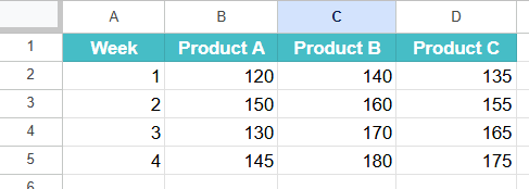
Step 1: Enter the weekly sales data in a Google Sheet as shown below. Each column represents a product, and each row shows weekly sales.

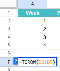
Step 2: Click on an empty cell, A7, and type the following formula:

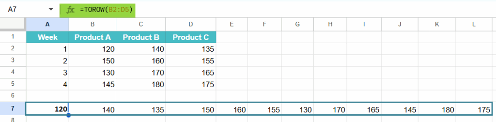
=TOROW(B2:D5)

Explanation:

• B2:D5 is the data range containing all the sales values.
• The TOROW function reads the range row by row and stacks all values into one horizontal list.

Step 3: Press Enter.
You’ll instantly see all the sales values displayed in a single row, listed one after another. This makes it easy to summarize, visualize, or share data in a compact format.

By using TOROW, the sales manager can quickly flatten the entire dataset into a single horizontal list. This saves time and minimizes manual data handling. It’s especially useful for preparing concise reports or dashboards.

Example #2 – Removing Blank Cells While Flattening Data

In this example, a research analyst is collecting data from multiple sources where some cells are left blank. The goal is to combine all values into one row while ignoring the empty cells. TOROW helps automate this process efficiently.

Step 1: Enter the data as shown below in your Google Sheet. Notice that some cells are blank.

Step 2: Click on an empty cell and enter the following formula:

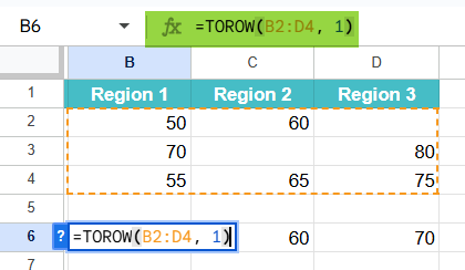
=TOROW(B2:D4, 1)

Explanation:

• B2:D4 is the range containing the data.
• The second argument 1 tells TOROW to ignore blank cells while flattening the data.

Step 3: Press Enter.
Google Sheets will instantly display all the non-blank values in one continuous horizontal line.

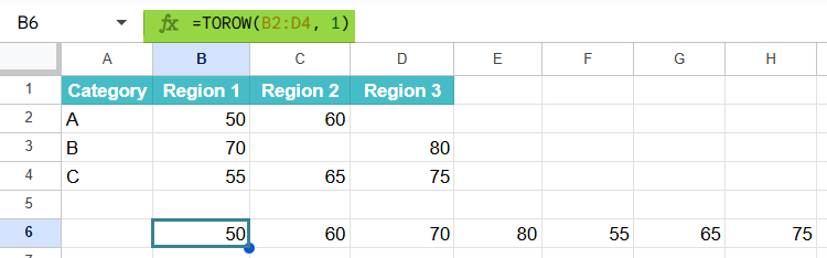
By using TOROW with the ignore blanks parameter, there is a clean, continuous row of data. This is very helpful for generating summaries or visualizations without any empty cells in the middle.

Example #3 – Combining TOROW with UNIQUE Function

In this example, an organization maintains a list of project codes assigned to different departments. Many projects overlap across departments, so there are duplicates. The goal is to create a single, unique list of all project codes in one horizontal row.

Step 1: Enter the project code data in your Google Sheet as shown below.

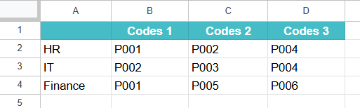
Step 2: To get the result, click on any empty cell and type the following formula:

=UNIQUE(TRANSPOSE(TOROW(B2:D4)))

Explanation:

• B2:D4 is the data range containing all the project codes.
• TOROW(B2:D4, 1) converts all values into a single row and removes blanks.
• UNIQUE filters out duplicate codes, leaving only one instance of each project code.
• Now, the TRANSPOSE can be confusing. The UNIQUE function expects its input array to be vertical by default. Google Sheets treats the entire horizontal array as one single row. Hence, to make UNIQUE work properly, you need to transpose the TOROW output so that UNIQUE sees it as a vertical list.

Step 3: Press Enter. The result will be a clean, horizontal list of all unique project codes.

One can use this function for creating summaries or lists from multiple departments. By combining TOROW with UNIQUE, users can quickly generate a duplicate-free dataset.

Important Things to Note

1. If you supply an invalid range or wrong argument type, Google Sheets will return a #VALUE! error.
2. The output of TOROW is a horizontal array that will automatically spill across adjacent cells to the right. Ensure those cells are empty.
3. Use the ignore parameter to skip blanks or errors (1, 2, or 3) for a cleaner row.
4. The scan_by_row parameter (default TRUE) determines whether values are read row-by-row; set it to FALSE to read column-by-column.
5. TOROW is exceptionally useful when preparing data for TEXTJOIN that require a single row.  It eliminates manual copying and reduces errors.

Frequently Asked Questions (FAQs)

Download Template

This article must help understand the TOROW Function in Google Sheets, with its formula and examples. We can download the template here to use it instantly.

Recommended Articles

Guide to What Is TOROW Function In Google Sheets. We explain how to use the TOROW Function In Google Sheets with examples and points to remember. You can learn more from the following articles. –

FACTDOUBLE in Google Sheets

UNICHAR in Google Sheets

SCAN in Google Sheets