
What is FACTDOUBLE in Google Sheets?
FACTDOUBLE in Google Sheets calculates the double factorial of a non-negative integer. Basically, it is the product of all integers from that number down to 1 that have the same parity, which is either even or odd. To use the function, one must enter the formula =FACTDOUBLE(A1). The argument can be a cell reference or number. For example, let us find the double factorial of the number 7. We enter the formula for the double factorial of 7 (7!!) is 7 × 5 × 3 × 1 = 105.
Thus, the FACTDOUBLE function computes the product of numbers with the same parity. It requires a non-negative integer as its argument. If you give negative numbers, it will result in an error. This function is often used in fields like probability theory and combinatorics.

Use this FACTDOUBLE in Google Sheets Template to follow along with the examples in this article.
Download Excel TemplateKey Takeaways
- FACTDOUBLE in Google Sheets calculates the double factorial of a number, written as n!!, multiplying either all even or all odd integers down to 1 or 2.
- The function is useful in probability, combinatorics, and advanced mathematics, especially when dealing with arrangements or outcomes restricted to odd or even numbers.
- The syntax of the FACTDOUBLE function is:
- =FACTDOUBLE(number)
- FACTDOUBLE only works with non-negative integers; using negative or decimal values will result in an error.
- If you need the regular factorial, use FACT; if you need double factorials for odd/even sequences, use FACTDOUBLE.
Syntax
The FACTDOUBLE in Google Sheets formula is as follows:
=FACTDOUBLE(value)
Here, value (required): This is the number for which you want to calculate the double factorial. It can be a positive integer or a cell reference containing a positive integer. If a non-integer value is provided, the decimal part will be truncated before calculation. We get an error if a non-numeric value is provided.
How To Use FACTDOUBLE Function in Google Sheets?
The FACTDOUBLE function in Google Sheets is used to calculate the double factorial of a number.
The double factorial of a number n (written as n!!) is the product of all integers from 1 to n that have the same parity (odd or even) as n.
- If n is even → product of all even numbers up to n.
- If n is odd → product of all odd numbers up to n.
It is useful in probability, and advanced mathematical calculations, especially when working with permutations and formulas in statistics.
To enter the FACTDOUBLE function in Google Sheets, there are two main ways:
- Enter FACTDOUBLE manually
- From the Google Sheets menu
Enter FACTDOUBLE Manually
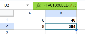
Let us look at the manual method to enter the FACTDOUBLE function. To illustrate this, we will calculate the double factorial of the number 6 and 8.
Here, the solution is 6!! = 6 × 4 × 2 = 48 and 8! = 8 × 6 × 4 × 2 = 384
Step 1: Open Google Sheets and in a new spreadsheet, enter the required numbers.

Step 2: Enter the FACTDOUBLE formula: in an empty cell (say B2).

Here, we start with an = sign, followed by the function name and open braces. Enter the argument inside the braces.
=FACTDOUBLE(A1)
Where A1 contains the number 6.
Step 3: Press Enter.
The cell B1 will display the result, which is 48.

Step 4: Now, drag the formula down to get the double factorial of 8.
Entering FACTDOUBLE Through the Menu Bar
- Go to the Insert tab. Choose Function → Math.
- From the list, select FACTDOUBLE.
- Enter the required argument.
- Press Enter to get the result.
For odd numbers like 7, FACTDOUBLE will calculate 7 × 5 × 3 × 1 = 105.
Examples
The primary purpose of FACTDOUBLE in Google Sheets is to calculate the double factorial of a number, which is the product of every second integer up to that number. It is commonly used in arrangements, probability, and advanced math problems. Let us look at three real-life examples.
Example #1
A person is planning a small event where 6 seats are arranged in a row. However, due to spacing rules, only every alternate seat can be occupied (i.e., 2nd, 4th, and 6th seats). To determine the number of ways this can be arranged mathematically, you can use the formula FACTDOUBLE in Google Sheets.
Step 1: In Google Sheets, enter the number of seats (6) in cell A1.

Step 2: In the result cell (B1), type the formula:
=FACTDOUBLE(A1)
Step 3: Press Enter. The result will be 48 (calculated as 6 × 4 × 2).

By applying FACTDOUBLE, we know there are 48 possible ways to arrange participants in every alternate seat.
Example #2 – Calculate the number of ways to arrange objects in groups
Suppose you have 9 identical objects and want to arrange them in groups, but only every second object is allowed in the arrangement (like selecting 1st, 3rd, 5th, etc.). Instead of multiplying the values manually, we can use FACTDOUBLE to simplify this grouping calculation.
Step 1: Enter the number of objects in cell A1.

Step 2: In cell B1, type:
=FACTDOUBLE(A1)

Step 3: Press Enter. The result will again be 945, representing the number of grouped arrangements.

FACTDOUBLE makes grouping calculations easier, giving us 945 ways to arrange objects in alternate groups. That’s a huge number of ways!
Example #3 – Calculate the probability of a specific outcome in a sequence of events
Consider a probability scenario where you roll a die multiple times but are only interested in odd-number outcomes. If you want the product of all odd outcomes up to 5 (i.e., 7, 5, 3, and 1), you need the double factorial of these numbers.
Step 1: Enter the numbers 1, 3, and 5 in Column A.

Step 2: In cell B1, type the formula:
=FACTDOUBLE(A1)

Step 3: Press Enter. The result will be as shown below

FACTDOUBLE in Google Sheets directly provides the results for the three odd numbers. It can be used in probability equations involving only odd-numbered outcomes.
Important Things to Note
- The function is very useful because it computes n!! (double factorial) quickly.
- It can only work with non-negative integers.
- FACTDOUBLE rounds down decimal numbers before calculation.
- It returns #NUM! error for negative values.
- If you input a decimal (e.g., 4.8), it rounds down the number before calculation.
Frequently Asked Questions (FAQs)
The double factorial is just like the factorial. However, here, instead of multiplying by each integer less than or equal to the provided value, the numbers decrement by 2. Thus, the double factorial of 5 is 15 and the double factorial of 7 is 105 (1* 3 * 5 * 7).
If a number or reference to a number is provided to FACTDOUBLE, the decimal part will be silently truncated before calculation.
The FACT function calculates the factorial of a number (n!), which is the product of all integers from 1 to n. For example, FACT(6) = 720. By contrast, FACTDOUBLE skips every alternate number. You would use FACT for general factorial calculations, while FACTDOUBLE is applied in more specialized scenarios like permutations, probability problems, and advanced math where only odd or even integers are relevant.
One common error is entering a negative number, which will return #NUM! because factorials are only defined for non-negative integers. Another issue arises if you input a non-integer value (like 5.5), which results in #VALUE! since FACTDOUBLE only works with whole numbers. Always ensure your input is a valid non-negative integer to avoid these errors.
FACTDOUBLE is often used in probability calculations (like rolling dice with odd outcomes), arrangement problems (like filling alternate seats), and in certain combinatorial formulas that specifically require even or odd factorials.
Use this FACTDOUBLE in Google Sheets Template to follow along with the examples in this article.
Download Excel Template