
What Is UNIQUE Function In Google Sheets?
The UNIQUE Function in Google Sheets checks the selected dataset’s row values, detects and discards the duplicate values. Then, it displays the extracted unique values as a new dataset. The Google Sheets UNIQUE function helps users to identify and remove the duplicate values in large datasets and have precise data while generating reports.
For instance, the following data consists of the items in order, but with some repeated ones that are highlighted.
Use this UNIQUE Function In Google Sheets Template to follow along with the examples in this article.
Download Excel Template
Select cell D2, enter the formula =UNIQUE(A2:A11) and press “Enter”, as shown below.

The output is shown above in the cells D2 to D8. Note, that the formula is entered in cell D2, however the duplicate values were removed and a new row is displayed in the output cells.
Key Takeaways
- UNIQUE Function in Google Sheets feature is a built-in function that will look for duplicates in columns and remove them to provide a new clear dataset.
- The function will extract only the unique records. However, if we want to filter non-duplicate values, we must set the last argument to TRUE.
- The dataset retrieved will be without formatting. We can format it as required once we get the final data to comprehend clearly.
- We must remember to apply the data validation to the main data and not the retrieved dataset. And, then select the new dataset for the criteria range.
- We can use the SORT function along with the UNIQUE function. The advantage is that when we retrieve the dataset without duplicates, then, we will have an alphabetically organized data for easy access.
Syntax
The syntax of the UNIQUE Google Sheets Formula is,

The arguments of the UNIQUE Google Sheets Formula are,
- range – It is the row’s cell range to be checked for or the entire dataset. It is the only mandatory argument in the formula.
- [by_column] – If we want to find a unique value from the column, we need to give the input as TRUE, and if we want to find duplicates from rows, then we need to give FALSE. Remember, FALSE is the default value if this argument is omitted. It is an optional argument.
- [exactly_once] – If we want to extract values appearing only once, we can use this argument by providing TRUE. By default, it will take FALSE as the input argument and extract distinct values.
How To Use UNIQUE Function In Google Sheets?
We can use the UNIQUE function In Google Sheets in 2 ways, namely,
- Access from the Google Sheets ribbon.
- Enter in the worksheet manually.
Method #1 – Access from the Google Sheets ribbon –
Step 1: Choose an empty cell for the output – select the “Insert” tab – click the “Function” option right arrow – click the “Text” option right arrow – select the “UNIQUE” function, as shown below.

Step 2: The “UNIQUE” formula appears, as shown below. Enter the argument as cell reference.

Method #2 – Enter in the worksheet manually –
Step 1: Select an empty cell for the output.
Step 2: Type = UNIQUE ( in the cell. [Alternatively, type =U or =UNI and double-click the UNIQUE function from the Google Sheets suggestions.]
Step 3: Enter the arguments as cell values or cell references and close the brackets.
Step 4: Press Enter to view the outcome.
Examples
Let us consider some examples to understand UNIQUE function in Google Sheets.
Example #1 – UNIQUE Function with multiple columns
Consider the data of the sales person and their regions and sales. We will use the Unique function to retrieve the unique values.

The steps to use the UNIQUE function with multiple columns are:
Step 1: Select cell E2 and enter the formula =UNIQUE(A1:C9), as shown below.

Step 2: Press “Enter” to get the retrieved dataset without any duplicate values, as shown below.

We can see that Row 2 and Row 6 are repeated with all the column values exactly the same. Hence, the formula discarded the duplicate row and displays the new dataset in the cells E2:G9.
Example #2 – UNIQUE function with SORT function
Let us consider the Example 1 dataset once again with the data of the sales person and their regions and sales. We will use the Unique function along with the SORT function to retrieve the unique values.

The steps to use the UNIQUE and the SORT functions are:
Step 1: Select cell E6 and enter the formula =SORT(UNIQUE(A2:B9)), as shown below.

Step 2: Press “Enter” to get the retrieved dataset in a sorted, organized manner, without any duplicate values, as shown below.

We can see that Row 2 and Row 6 are repeated with all the column values exactly the same. Hence, the formula discarded the duplicate row and displays the new dataset the first column displayed in an alphabetical order in the cells E2:G9.
Example #3 – UNIQUE function with horizontal data
The following table consists of the cosmetics brands campaign data given below with their region and sales. We will use UNIQUE function with horizontal data to discard duplicate values. Please note that, by default, the UNIQUE function checks the columns to find duplicate values, but when we use TRUE, it changes direction and checks across the rows.

The steps to use the UNIQUE function with horizontal data are:
Step 1: Select cell B10 and enter the formula =UNIQUE(A2:G5,true) as shown below.

Step 2: Press “Enter” to get the retrieved dataset without any duplicate values, as shown below.

Example #4 – Create Drp-Down Menus from lists with UNIQUE
We have a list of topics with their ID’s which are discussed in seminar session. We will first use the UNIQUE function to discard the duplicates and then Create Drop-Down Menus.

The steps to Create Drop-Down Menus from Lists with UNIQUE are:
Step 1: Select cell D2. Now, and enter the formula =UNIQUE(B1:B11) as shown below.

Step 2: Press “Enter” to get the retrieved dataset without any duplicate values. It is as shown below.

Step 3: Now, that we have the retrieved list, let us create a drop-down.
First, choose the cells B2:B11, to apply the drop-down– select the “Data” tab – click the “Data validation” option. The “Data validation rules” window opens on the right and click the “Add rule” option, as shown below.

Step 4: Let’s add the rule. Click the “Criteria” option drop-down and select the “Dropdown(from a range)” option, as shown below.

Step 5: Select the criteria range as D3:D8, as shown below in the “Select a data range” pop-up.

Step 6: Select the colors as required for color coding and click the “Done” option.

We have the final dataset with the drop-downs with different colors, as shown below.

By using this method, we can efficiently organize data and the resource allocation process for various workshops is simplified, easy and time saving.
Important Things To Note
- While dealing with multiple columns to UNIQUE Function, Google Sheets will look for duplicates in each column of all rows.
- We get the #REF error if we do not have enough space to retrieve the values.
Frequently Asked Questions (FAQs)
We often forget in which category a function falls, here, the “UNIQUE” function. Then, we can insert the function as follows:
Choose an empty cell – select the “Insert” tab – click the “Function” option right arrow – click the “All” option right arrow – select the “UNIQUE” function, as shown below.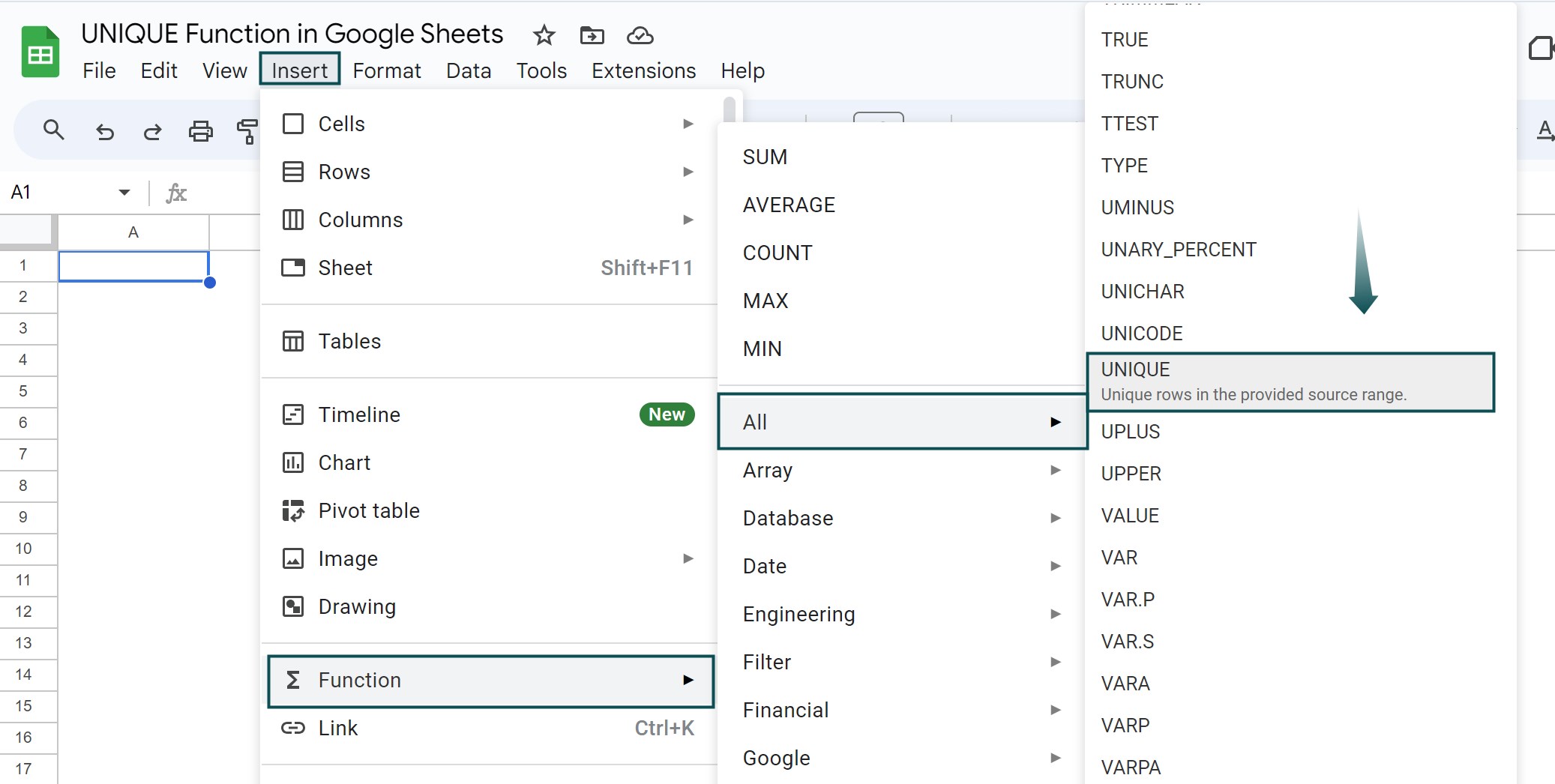
However, as always, entering the function manually is the best way to avoid confusion.
Alternatively, we can find the Functions icon to insert the UNIQUE function in Google Sheets by following the path shown below.
Choose an empty cell – click the “More” option represented by the three vertical dots at the end of the toolbar, as shown below.
A list of icons appears when we click the “More” option. Here, click the “Functions” icon, as shown below.
Here, click the “Functions” option – click the “All” option right arrow – select the “UNIQUE” function, as shown below.
The UNIQUE function in Google Sheets is will give an error for the following reasons;
a. If we are looking in horizontal data and not applied True in the formula.
b. Only the first column gets retrieved and not the other columns.
c. The formula is not applied for the right range.
Use this UNIQUE Function In Google Sheets Template to follow along with the examples in this article.
Download Excel Template