What is Excel VBA Filter?
The Excel VBA Filter is a robust tool that lets you automate the data filtering process. It is a component of Excel’s VBA programming which lets you manipulate different Excel operations programmatically. You can efficiently handle big data sets by applying filters which will only show and sort information that satisfies predetermined standards.
Let us look at an example where we apply a text-based filter in Excel using VBA. The “FilterByText” subroutine in this example is intended to VBA filter data in the range of A1 to D10.
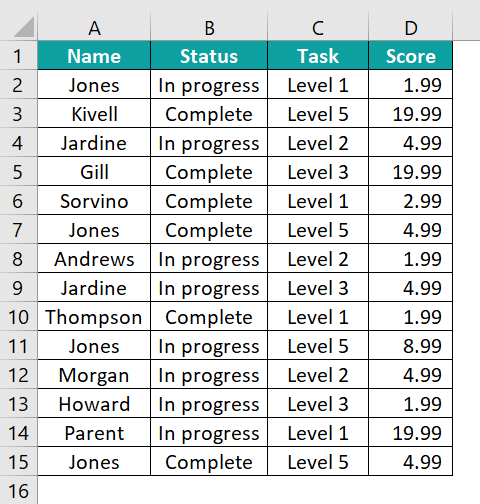
This range covers columns A through D and rows 1 through 10. This filter focuses on Column B, the second column, which we presume has status information.

By using Criteria1:=”Complete”, the filter specifically targets rows with the text “Complete” in the second column, simplifying data management and review.
When you run this code, it filters the data to display only those rows in Column B with the status “Complete” indicated when it is run.
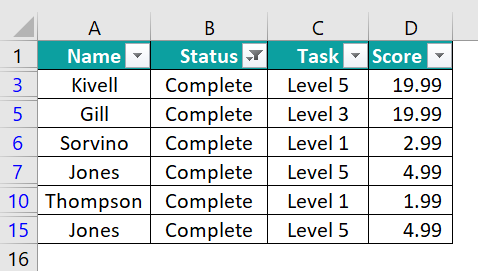
Table of contents
Key Takeaways
- Data filtering tasks can be effectively automated with VBA filter Data.
- Accurately defining the criteria and range in the VBA code is essential.
- Complex data scenarios can be handled with the help of advanced filtering options.
- Don’t forget to reset the view of your data by clearing the filters.
Excel VBA 5-in-1 Course Bundle – (30+ Hours of Expert-Led Training)
If you want to learn Excel and VBA professionally, then the Excel VBA 5-in-1 Course Bundle (30+ hours) is the perfect solution. Whether you’re a beginner or an experienced user, this bundle covers it all – from Basic Excel VBA to Event Automation, Error Handling, Email Automation, and real-world applications with downloadable templates.
How to Use Excel VBA Filter?
To use VBA Filter Data, follow these steps:
- Open Excel and press ALT + F11 to open the VBA editor.

- Insert a new module by clicking on “Insert” in the menu and selecting “Module.”

- Start writing your VBA code in the module for Filtering.
For example, to write something like this to filter a range of data based on specific criteria:
Range("A1:B10").AutoFilter Field:=1, Criteria1:="YourCriteria"
This example sets a filter on the first column (Field:=1) of the range A1:B10 for a specified criterion (“YourCriteria”). The AutoFilter function in Excel VBA requires an understanding of its syntax and parameters in order to be used effectively.
AutoFilter Syntax and Parameters:
- Run the VBA Code by pressing F5 or by clicking on the Run button in the VB editor.
Examples to Filter Data Using VBA
Example #1 – Apply or Remove Filter to the Data
Let’s say you want to use VBA Filter Data to apply a filter to some Excel data. We’ll see how to accomplish this in this example.
- Step 1: Supply Data Range
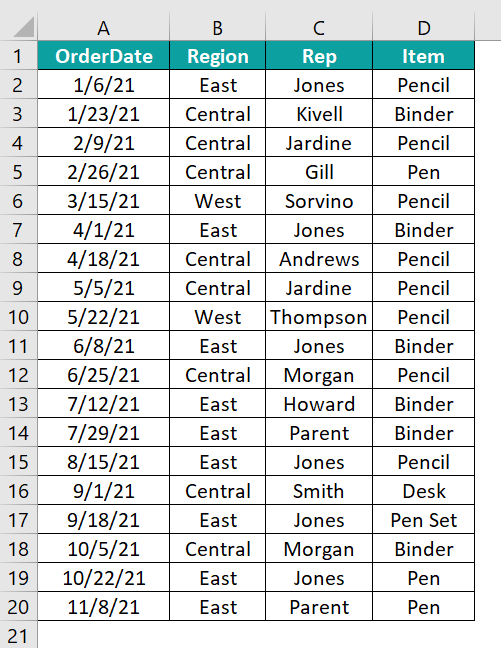
The first line of the code is Range (“A1:D10”). The data range that the filter will be applied to is specified on this line. The range in this case is cell A1 to cell D10.
Thus, all the data in rows 1 through 10 and columns A through D will be subject to the filter. Your data must fall inside this range for the filter to function properly.

- Step 2: Access AutoFilter Function
The “.AutoFilter” is then applied to the designated range. For the specified range, this section of the code activates the AutoFilter feature in VBA.
The user can filter the data according to their needs by using the AutoFilter method, which displays a dropdown in the header row for each column in the designated range. This line of code will remove any filters that are already applied to the range.

- Step 3: Run the Code to Enable the Filter
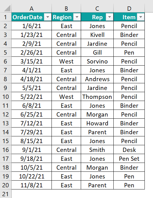
The entire code is wrapped within a sub-procedure named “ApplyRemoveFilter().” This is a custom VBA subroutine. Running it will trigger the actions defined in the steps above. When you run this macro, you will see that the filter has been applied to the columns.
Here is the full code:
Sub ApplyRemoveFilter()
Range(“A1:D10”).AutoFilter
End Sub
Example #2 – Filter Specific Values
This example shows how to apply a VBA filter to data within a given range, to display only rows in which the value in the first column matches.
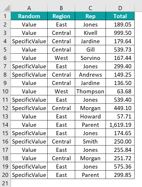
- Step 1: The code begins with Range(“A1:D20”).AutoFilter. This line designates the A1:D20 data range that the filter will be applied to.
It indicates that every piece of information from column A to column D and rows 1 through 20 has been chosen. Then, on this range, the AutoFilter method is called, allowing the filtering options to be used.

- Step 2: The column number that the filter is to be applied to is specified by “Field:=1” in the same line.
“Field:=1” in this instance indicates that the filter is being applied to the first column of the range that has been chosen, in this case, column A. Here is where the filtering criteria will be used.

- Step 3: The filtering criterion is defined using “Criteria1:=”SpecificValue”” after the field selection. Here, the value “SpecificValue” is being used to filter the first column (Field 1).
After the filter is applied, only rows with column A’s value of “SpecificValue” will be displayed. This value can be changed to any other value as needed.

- Step 4: The “FilterSpecificValues” subroutine applies an AutoFilter to the range A1:D20 when it is executed, displaying only rows where Column A’s value is “SpecificValue” and concealing all other rows.
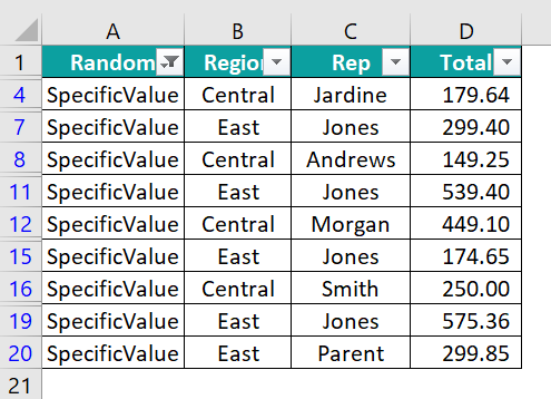
Here is the full code:
Sub FilterSpecificValues()
Range(“A1:D20″).AutoFilter Field:=1, Criteria1:=”SpecificValue”
End Sub
Example #3 – Usage of OPERATOR Argument
This example demonstrates the use of VBA Filter data to target rows in range A1:D15 where the second column simultaneously satisfies two requirements by having both “Math” and “Politics” in it.
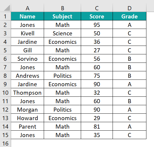
- Step 1: The first line of code is “Range(“A1:D15″).””AutoFilter.” This line indicates the range of data that the “AutoFilter” will be applied to, which is cells A1 through D15. All data in rows 1 through 15 and columns A through D are included in the range.
“Field:=2” is specified right after the range. This means that the first field (or column) of the chosen range—in this case, column B—will be subject to the filtering criteria.

- Step 2: Here, we define “Criteria1:=”Math”.” This section of the code establishes the initial filtering criterion for the first field (column B). Rows with “Math” as the value in column B will be filtered out.

- Step 3: “Operator:=xlOr” is introduced after the first criterion. Because it controls how the two criteria will interact, this operator is very important.
In this case, xlOr means that either of the criteria must be met for a row to be displayed after the filter is applied.

- Step 4: Criteria2:=”Politics” is finally set. This is the filter’s second requirement. This criterion is used in conjunction with the first one using the “xlOr” operator.

- Step 5: When you run the FilterUsingOperator subroutine, it applies a filter to range A1:D15 on the second column, showing only rows where values in Column B are both “Math” or “Politics”.

Here is the full code:
Sub FilterUsingOperator()
Range(“A1:D15″).AutoFilter Field:=2, Criteria1:=”Math”, Operator:=xlOr, Criteria2:=”Politics”
End Sub
Example #4 – Filter Numbers with operator Symbols
In this example, we will see how to use VBA Filter Data to apply filters to the data with two criteria and an operator to filter data that is more than 10 and less than 20.
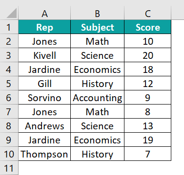
- Step 1: In the new module, we first start by creating a new subroutine named FilterNumbers.

- Step 2: In this line, we apply the AutoFilter:
Range(“A1:D10”).AutoFilter: The range on the worksheet from cell A1 to D10 is chosen by this section of the code.
Next, a filter is applied to this range using the “.AutoFilter” method. This indicates that you are filtering the information in the first ten rows of columns A through D.

- Step 3: Now, we specify the Filter Criteria for the First Field:
Field:=3: This indicates that the first field (or column) in this range, which is Column C, is where the filter should be applied.
Criteria1:=”>10″: This establishes the filter’s initial criterion. Excel is instructed to only display rows when the value in Column C exceeds 10.

- Step 4: Here, we will use an Operator to combine the two criteria.
Operator:=xlAnd: The two criteria are combined using this operator. This indicates that for a row to be displayed, both requirements must be satisfied.

- Step 5: In this step, we specify the second filter criteria.
Criteria2:=”<20″: This establishes the filter’s second requirement. It tells Excel to restrict the visible rows even further to those where Column A’s value is likewise less than 20.

- Step 6: When you execute this code, you will see that Column C is filtered with our required criteria and only the fields that satisfy our requirement are populated.
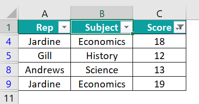
Here is the full code:
Sub FilterNumbers()
Range(“A1:C10″).AutoFilter Field:=3, Criteria1:=”>10″, Operator:=xlAnd, Criteria2:=”<20″
End Sub
Example #5 – Apply Filter for More Than One Column
This example will demonstrate how to apply the VBA filter data to two distinct columns in the range A1:D20, displaying rows in which “East” appears in Column A and “Jones” appears in Column B.
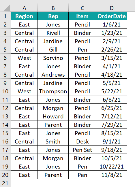
- Step 1: Start by creating a new VBA subroutine named FilterMultipleColumns.

- Step 2: In this line, we apply the AutoFilter to the First Field:
Range(“A1:D20”): Select the data range from cell A1 to D20 on the worksheet.
.AutoFilter: Applies the AutoFilter method to the selected range.
Field:=1: Specifies that the filter should be applied to the first field (Column A in this case).
Criteria1:=”East”: Sets the filter condition for Column A to display only the rows where the value is “East”.

- Step 3: Now, we apply the AutoFilter to the Second Field:
“Range(“A1:D20”).AutoFilter Field:=2, Criteria1:=”Jones””: This line repeats a similar process for a different column:
It again selects the same range (A1:D20).
Field:=2: Indicates the filter is now being applied to the second field, which is Column B.
Criteria1:=”Jones”: Sets the filter condition for Column B to show only rows where the value is “Jones”.

- Step 4: Save the module and run the code. When this code runs, it first shows only rows where the value is “East” by filtering the data in Column A within the range A1:D20.
It instantly applies a second filter to Column B within that same range, limiting the number of rows to those with the value “Jones”. As a result, only rows that satisfy both requirements are shown.
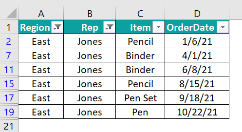
Here is the full code:
Sub FilterMultipleColumns()
Range(“A1:D20″).AutoFilter Field:=1, Criteria1:=”East”
Range(“A1:D20″).AutoFilter Field:=2, Criteria1:=”Jones”
End Sub
Important Things to Note
- VBA filter data based on cell value ensures that the data type in the cell used for filtering matches the data type in the column being filtered.
- For VBA filter data and copy to another sheet, it’s essential to correctly select the filtered range using “Range.SpecialCells(xlCellTypeVisible)” before copying to ensure only visible, filtered data is transferred.
- VBA filter data based on dropdown selection ensures the filtering action dynamically responds to the dropdown changes, typically using the “Worksheet_Change” event.
- Make sure your code can adjust to different data ranges and can handle changes in the size or structure of the data without requiring manual adjustments when using VBA filter data.

Frequently Asked Questions (FAQs)
In Excel VBA, “advanced filter data” refers to filtering methods that surpass simple filtering, like applying multiple criteria, intricate logical operators, or filtering across multiple sheets.
In Excel VBA, choose the data range and use the “.AutoFilter” method with the relevant field and criteria parameters to enable auto filtering.
Use the “.AdvancedFilter” method on the desired range and the “Unique:=True” parameter in Excel VBA to filter duplicate data.
In Excel VBA, deselect a filter by applying the “.AutoFilter” method to the range where the filter is applied without any parameters.
Download Template
This article must be helpful to understand the VBA Filter Data, with its examples. You can download the template here to use it instantly.
Recommended Articles
A guide to VBA Filter Data. Here, we learn to filter data in Excel VBA in different ways like using specific filters with suitable examples. You can learn more from the following articles –


Leave a Reply