
What Is Vlookup To Return Multiple Values In Google Sheets?
The VLOOKUP to return multiple values in Google Sheets is an array formula that searches for one or more search keys in a specific range. Once it finds one or more matches for the search keys, the function lists all the return values corresponding to the search key matches from the lookup range.
Users can use the Google Sheets formula to vlookup to return multiple values when they must find all the values associated with a specific item when managing inventory at a store or reviewing survey results.
Use this Vlookup To Return Multiple Values In Google Sheets Template to follow along with the examples in this article.
Download Excel TemplateFor example, the source dataset lists sales representatives and their monthly salaries from January to March.

We must update the three months’ salaries for the representative mentioned in cell A12 and display the outcome in cells B12:D12.
Then, we can apply the VLOOKUP()-based ARRAYFORMULA() in the target cells, considering the meaning of the vlookup to return multiple values in Google Sheets explained previously.

The VLOOKUP() executes as an array formula as we nest it within the ARRAYFORMULA(). The VLOOKUP(), like the Excel VLOOKUP function, searches for an exact match for the representative, cited in cell A12, in the first column of the search range A2:D9. It finds the match in cell A5, which is in row 4 of the range A2:D9. Next, it returns the salaries in row 4 of columns B, C, and D, indicated by the array of indices {2,3,4}, which are the cells B5:D5 values.
Thus, the array formula, applied in cell B12, shows the three salary values that the function VLOOKUP to return multiple values in Google Sheets returns in the three adjacent cells B12:D12.
Key Takeaways
- The formula VLOOKUP to return multiple values in Google Sheets enables us to find the matches for one or more search keys and accordingly secure the corresponding return values from the specified range.
- Users can use the Google Sheets formula to vlookup to return multiple values when they must search multiple search keys and retrieve multiple corresponding values. The function also helps to secure all the values from the matching row by using multiple-column indices.
- The alternative to the VLOOKUP()-based ARRAYFORMULA function, which returns multiple values, is to use the INDEX()-based ARRAYFORMULA function. Otherwise, we can use COUNTIF() to generate unique search keys in a helper column. After that, we can apply the VLOOKUP() in the target cell, based on the search key with the same format as the values in the helper column. Further, we can also use the FILTER() as an alternative.
How To Return Multiple Values Using VLOOKUP Function In Google Sheets?
The steps to return multiple values using the VLOOKUP function, in line with the definition of VLOOKUP to return multiple values in Google Sheets explained earlier, are as follows:
- Select a cell to showcase the output.
- Enter the applicable VLOOKUP() nested within the ARRAYFORMULA().
When we have multiple search keys, and we must retrieve multiple corresponding values, use the following formula:
=ARRAYFORMULA(VLOOKUP(search_keys_range, range, index, [is_sorted]))
Where,
- search_keys_range: The reference to the cell range holding the values we must find the matches for in the search range.
- range: The range where we must look for a match for the search keys and which includes the column holding the potential return values.
- index: The index of the column holding the potential return values in the cited range. Also, the argument value should be a positive integer.
- is_sorted: The argument value is TRUE (or 1) or FALSE (or 0). The recommended value is FALSE, denoting an exact match for the search keys. In contrast, the default value of the argument is TRUE, indicating an approximate match for the search keys. It implies that when we omit this argument value, the VLOOKUP() considers the argument’s default value.
Furthermore, when we want the function to find an approximate match for the search keys, the search keys in the first column of the cited range should be sorted in ascending order. Otherwise, the function may return an incorrect value.
When we must use the VLOOKUP() to retrieve all the values from the matching row (utilizing multiple column indices), apply the following formula:
=ARRAYFORMULA(VLOOKUP(search_key, range, indices_array,[is_sorted]))
Where,
- search_key: The value or reference to the cell holding the value we must find the match for in the search range.
- range: The range where we must look for the matches for the search key and which includes the columns holding the potential return values.
- indices_array: The array of indices of the columns containing the potential return values in the cited range. Also, the array should contain positive integers.
- is_sorted: The argument definition is the same as mentioned earlier.
- Press Enter to view the output that the array formula VLOOKUP to return multiple values in Google Sheets returns in the target cell and the cells adjacent to it. The target cell count will depend on the output array size.
Examples
The illustrations below show the practical ways of using VLOOKUP to return multiple values in Google Sheets.
Example #1
The source dataset shows the store location-based yearly inventory level data from 2020-23.
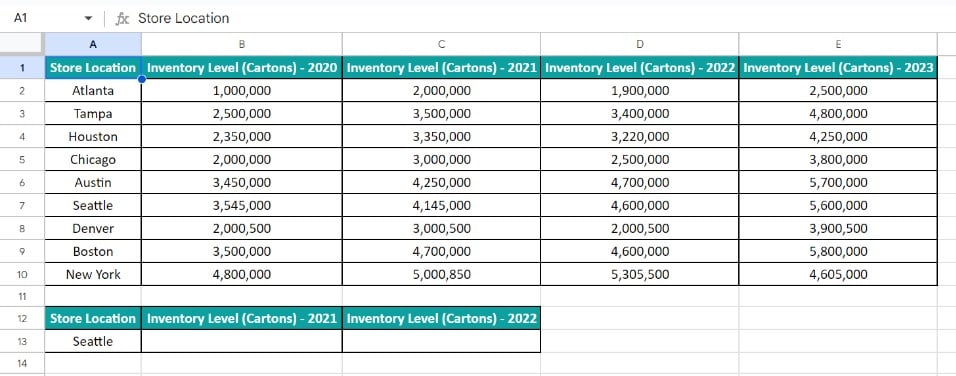
We need to update the 2021 and 2022 inventory level data for the store location, Seattle, cited in cell A13. Assume cells B13:C13 are the target cells.
We can secure the required data using VLOOKUP to return multiple values in Google Sheets formula in the target cells.
Step 1: Select cell B13, enter the ARRAYFORMULA() containing the VLOOKUP(), and press Enter.
=ARRAYFORMULA(VLOOKUP($A$13,$A$2:$E$10,{3,4},0))

We want the VLOOKUP() to return multiple values. So, we must use multiple column numbers (index) within curly braces when supplying the VLOOKUP to return multiple values in Google Sheets arguments, as mentioned below:
{3, 4}
It creates an array that returns multiple column values, which are the values from columns 3 and 4 of the search range.
Furthermore, we have used curly braces to achieve an array within the VLOOKUP(). However, the VLOOKUP() does not execute as an array formula by default. Thus, we must nest the concerned VLOOKUP() in the ARRAYFORMULA(). So, the final array formula is the following:
=ARRAYFORMULA(VLOOKUP($A$13,$A$2:$E$10,{3,4},0))
The VLOOKUP() searches for the cell A13 value, Seattle, in the first column of the range A2:E10. It locates an exact match for the search key in cell A7, which is in row 6 of the range A2:E10. Next, the index in the VLOOKUP() is an array of positive integers, 3 and 4. So, the function returns the values in row 6 of columns C and D in the range A2:E10, which are the cells C7 and D7 values, 4,145,000 and 4,600,000.
Furthermore, the expression executes as an array formula. So, we get an array of two column values (cells C7 and D7 values) as the output in cells B13:C13.
Example #2
The source dataset contains employees’ first and last names, and their teams.

The task is to show the teams in column H that have an employee with the first name Fred, as cited in cell G2.
Step 1: Consider column A as the helper column. We shall populate it with unique search keys required to perform a vlookup to return multiple values in column H.
So, select cell A2, enter the following expression, and press Enter.
=C2&B2

Next, use the option of fill handle to populate the formula in the remaining column A cells.

We concatenate each employee’s first name and their corresponding serial number to create a list of unique search keys in the helper column.
Step 2: Select cell H2, enter the ARRAYFORMULA() containing the ROW() and VLOOKUP() within the IFERROR(), and press Enter.
=ArrayFormula(IFERROR(VLOOKUP(G2&ROW(A1:A11),$A$2:$E$11,5,FALSE),””))

Let us see the explanation for the VLOOKUP to return multiple values in Google Sheets arguments specified in the formula mentioned above to understand its logic.
First, the ROW(A1:A11) returns an array of values 1 to 11. So, the term G2&ROW(A1:A11) combines the cell G2 value and the ROW() (with the same logic as the Excel ROW function ) output to generate the search keys Fred1, Fred2, and so on till Fred11.
Next, the VLOOKUP() looks for the exact matches for the search keys in the first column of the search range A2:E11. It finds the exact matches in cells A3, A5, A6, and A8 for the search keys Fred2, Fred4, Fred5, and Fred7, respectively. So, the function output is the values in the corresponding rows 2, 4, 5, and 7 of column E in the range A2:E11.
The VLOOKUP() executes as an array formula. So, we see the values the function returns for the corresponding matches of the search keys in the respective rows 2, 4, 5, and 7 of column H in the range H2:H11. However, the remaining cells in the range H2:H11 will show the #N/A error. The reason is that the VLOOKUP() does not find the match for the concerned search keys in the search range and returns the #N/A error. So, we nest the VLOOKUP() within the function IFERROR in Google Sheets, which works like the function IFERROR in Excel, to check if the value that the VLOOKUP() returns is an error value. In such a case, the IFERROR() replaces the error value with a space character.
Example #3
The source dataset contains a clients list and their contact numbers.

We must update the contact numbers of the clients listed in column D and display the output in column E.
Step 1: Select cell E2, enter the ARRAYFORMULA() containing the VLOOKUP(), and press Enter.
=ARRAYFORMULA(VLOOKUP(D2:D5,A2:B11,2,0))

The VLOOKUP() accepts the range D2:D5 as the search keys range. Next, the search range is A2:B11, and the index, 2, of column B holding the potential return values in the search range is supplied as the third argument. Finally, the last argument value, 0, indicates the function must perform an exact match.
So, the function looks for the exact matches for the four clients, cited in cells D2:D5, in the first column of the range A2:B11. It locates the matches in cells A8, A6, A2, and A10 (rows 7, 5, 1, and 9 of the range A2:B11). So, the function executes as an array formula and returns the values in rows 7, 5, 1, and 9 of column B in the range A2:B11, which are the cells B8, B6, B2, and B10 values. Thus, the array formula output gets populated in the target range E2:E5.
Alternative Methods To Return Multiple Values
The first alternative method to return multiple values in Google Sheets involves the INDEX() implemented as an array formula.
The steps are as follows:
- Choose the target cell to display the output.
- Enter the INDEX() nested within the ARRAYFORMULA().
=ARRAYFORMULA(IFERROR(INDEX(return_values_range_absolute_reference,SMALL(IF(search_key=search_range_absolute_reference,ROW(search_range_absolute_reference)-ROW(search_key)+1), ROW(1:1))),””)) - Press Enter to execute the formula.
- Utilize the fill handle to update the formula in the remaining target cells.
For example, the source dataset lists a set of stocks and their daily prices.

The requirement is to update the prices of the stock, cited in cell E2, in cells F2:F5.
Step 1: Select cell F2, enter the following formula, and press Enter.
=ArrayFormula(IFERROR(INDEX($C$2:$C$11,SMALL(IF($E$2=$A$2:$A$11,ROW($A$2:$A$11)-ROW($A$2)+1),ROW(1:1))),””))

Next, utilizing the fill handle, which works like the Excel fill handle, feed the formula in cells F3:F5.

The second method involves the COUNTIF(), similar to the Excel COUNTIF function, and the VLOOKUP().
The steps are as follows:
- Firstly, insert a column at the start of the source dataset and name it the Helper Column.
- Next, select the first cell in the helper column, enter the required COUNTIF(), and press Enter to secure the unique search keys.
=COUNTIF(source_dataset_first_cell_absolute_reference:source_dataset_first_cell_reference, source_dataset_first_cell_reference)& source_dataset_first_cell_reference - Utilize the fill handle to implement the formula in the remaining helper column cells.
- Please choose the first cell in the target range, where we must display the return values. Next, enter the VLOOKUP(), and press Enter.
=VLOOKUP(search_key&unique_count,range,index,[is_sorted]) - Use the option of fill handle to apply the formula in the remaining target cells.
For example, the first dataset lists stationery items, their categories and costs.

We must update the stationery items’ costs in column I of the second table based on the first table data.
Step 1: Column A in the first dataset is the helper column and it is empty.
So, choose cell A2, enter the COUNTIF(), and press Enter.
=COUNTIF($B$2:B2,B2)&B2

Next, with the help of the fill handle, update the expression in the remaining helper column cells.

Next, column G of the second dataset contains the count of each stationery item’s occurrence. It is required to create unique search keys in the same format as the helper column values.
Step 3: Select cell I2, enter the VLOOKUP(), and press Enter.
=VLOOKUP(G2&F2,$A$2:$D$10,4,0)

Next, enter the function in the remaining target cells with the help of the fill handle.

Important Things To Note
- When using the function VLOOKUP to return multiple values in Google Sheets, nest it within the ARRAYFORMULA() to execute it as an array formula.
- Assume the VLOOKUP function, implemented as an array formula to secure multiple values in Google Sheets, does not find any matches for the search key. Then, the function output is the #N/A error.
Frequently Asked Questions (FAQs)
We can vlookup to return multiple values in Google Sheets using the FILTER() as described below with an example.
The source dataset shows a set of products and their quarterly units sold data.
The need is to display the units sold data for the product specified in cell E2 in all quarters in column F.
Step 1: Select cell F2, enter the FILTER(), and press Enter.
=FILTER(C2:C13,E2=A2:A13)
The FILTER() returns an array of the required values, which are displayed in the range F2:F5. The function accepts two inputs. The first is the range holding the potential return values. On the other hand, the second is the condition the function must check.
So, the function checks for the product, Smartphone, cited in cell E2, in the range A2:A13. It finds matches in cells A3, A6, A9, and A12. So, the function returns the values in the corresponding rows of column C, which are the cells C3, C6, C9, and C12 values, as the required output.
We can handle the #N/A errors when using VLOOKUP for multiple values in Google Sheets by nesting the VLOOKUP() in the IFERROR(). The IFERROR() helps to display a customized output instead of the error value.
There is no limit to the number of values VLOOKUP may return in Google Sheets. We can use the function to return as many matching values as there are in the source dataset.
Use this Vlookup To Return Multiple Values In Google Sheets Template to follow along with the examples in this article.
Download Excel Template