
What Is What-If Analysis in Google Sheets?
What-if analysis is a type of analysis in Google Sheets through which you can plug different numbers into formulas to observe the change in the results. What-if analysis is a powerful decision-making tool to help users explore different results that are obtained by changing the input values in the given formulas. Google Sheets makes this process easier by offering tools like Goal Seek.
Here, we can test various scenarios without altering the core data. Thus, it is useful in areas like forecasting, budgeting, and problem-solving. They can adjust one or more variables to see how those changes affect the results. It is very helpful in strategic planning and data-driven decisions.
Use this What-If Analysis in Google Sheets Template to follow along with the examples in this article.
Download Excel TemplateFor example, a small business owner may want to observe how adjusting product prices will affect their profit. To do so, he can set up a spreadsheet where he uses formulas and use the What-If Analysis to adjust the prices. The sheet will automatically update the calculations using tools like Goal Seek.

Key Takeaways
- The What-If Analysis in Google Sheets helps you learn how changing the input values affects the results in your spreadsheet formulas, making it an important tool for decision-making.
- Goal Seek is used to find the required input to reach a specific output by automatically adjusting one variable for multiple iterations till the goal is reached.
- One must install Goal Seek from the Add-ons menu under Extensions > Add-ons > Get add-ons.
- It is especially useful for financial planning, forecasting and testing of scenarios with a single changing variable.
How To Perform What-If Analysis with Goal Seek in Google Sheets?
Goal Seek in Google Sheets is a tool used that is used for the What-If Analysis. It can be used to find the right input value to achieve a desired result. It works by adjusting a variable in the spreadsheet with different values until the formula reaches the target value we specify. This enables one to predict outcomes and make calculated decisions.
Let us look at the steps to perform a What-If Analysis in Google Sheets using Goal Seek.
Step 1: First, we set up our formula. For this, we start entering a formula in a cell with a value that is dependent on another cell. In this example, we have cell A2 with the quantity, B2 with the price, and C2 as total revenue with the formula =A2*B2.

Step 2: Now, let us access Goal Seek – Google Sheets by following these steps.
To install Goal Seek, go to
Extensions -> Add-ons -> Get add-ons.
Now, in the search bar, search for “Goal Seek,” and install it.


The tool gets installed!

Step 3: Click on Extensions -> Goal Seek -> Open.

Step 4: In the Goal Seek sidebar, we enter the following details.
Set “Set cell” to the cell that contains the result you want to achieve. Here, it is cell C2.
Next, set “To value” to the target result we need. Here, it is $2000.
Finally, we set “By changing cell” to the input variable we wish to adjust. A2 is entered here.
Step 5: Now, let us run Goal Seek. For this, click on Solve, shown above, and Google Sheets will adjust the input cell to find a value that makes the result match your target value.

For this, Goal Seek will try various values in cell A2 until it’s able to achieve the value of 2000 in cell D5.

Goal Seek Parameters
The different parameters available in Goal Seek include:
- Set cell: It is the cell that contains the formula where you wish to reach a specific value. It must be dependent on another cell.
- To value: It is the target value you want the “Set cell” to achieve. This is the goal you are looking to reach.
- By changing cell: This is the input cell that Goal Seek will adjust to reach the set target value. It should have a dependency on the the “Set cell” via a formula.
Examples
Let us look at some examples where we use the What-If Analysis in Google Sheets. This is very similar to the What-if Analysis in Excel.
Example #1 – Predict Monthly Loan Payments Based on Different Interest Rates and Loan Terms Using What-If Analysis with Goal Seek
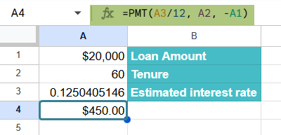
In this example, a person is planning to take a $25,000 loan They wish to know what interest rate would result in a monthly payment of $450 over a 5-year term. It is very hard to manually try different interest rates. Instead, one can use Goal Seek in Google Sheets to find the exact rate that meets the target payment.
Step 1: Go to a spreadsheet and enter the details as follows. Enter the loan amount in cell A1 as 25000, the loan term in months in A2 as 60, and an estimated interest rate in A3 (e.g., 5% or 0.05).
Step 2: We type the following formula in cell A4.
=PMT(A3/12, A2, -A1)
to calculate the monthly payment.
Step 3: Now, to use Goal Seek, go to Extensions -> Goal Seek -> Open.
Step 4: In the Goal Seek sidebar, set the following values. Enter the “Set cell” value as A4 (the monthly payment), the “To value” as 450 (your desired monthly payment), and “By changing cell” as A3 (the given interest rate).

Step 5: Click on Solve. Goal Seek will find the interest rate that results in a $450 monthly payment.

Thus, the annual rate is 12.5% for getting a monthly payment of $450.
This method quickly identifies the required interest rate by using different values till it matches the set target value. Thus, Goal Seek simplifies financial planning by adjusting the inputs to meet specific financial goals.
Example #2 – Determine the Minimum Number of Course Enrolments Needed to Break Even
Goal Seek can be used to determine break-even requirements in business when all other parameters are known. Suppose a person is offering an online yoga course that costs $50 per enrolment. They have fixed costs of $1,500 for aspects like marketing, etc. They want to know how many students should enroll to break even which means to cover all the costs with the revenue earned.
Step 1: In a spread sheet, enter the fixed cost in cell B1 as $1500. The, enter the course price per student in cell B2 as $50. As before, enter a guess for the number of enrolments in B3. Here, we enter 10.
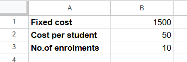
Step 2: In cell B4, they calculate the revenue using the formula =B2*B3.(students*cost per enrolment).
In cell B5, we calculate the profit using the formula =B4-B1.

Step 3: Now, open Goal Seek. Go to Extensions > Goal Seek > Open.

Step 4: In the side bar, set the “Set cell” as A5 (profit), “To value” as 0, which is the break-even point, and “By changing cell” as A3, which is the number of enrolments.

Step 6: Click on Solve. Goal Seek will calculate the minimum number of enrolments needed to cover your costs.

The number of required enrolments to break even is 30. Thus, one can use Goal Seek to find how many enrolments are needed to avoid a loss. It is a practical way to test pricing strategies.
Goal Seek finds a solution within the parameters given.
Example #3 – Explore Multiple Salary Raise Scenarios to Estimate Future Income
To explore multiple salary, raise scenarios and estimate future income, one can use Google Sheets’ “What-If Analysis” tool, specifically Goal Seek. This tool helps determine what input value is needed to achieve a desired outcome. For instance, what salary raise percentage is needed for an annual income.
Step 1: Let us infer that the current salary is $120,000, and we wish to reach a $180,000 annual income in 3 years.
- Enter the current salary of $120,000 in cell B1.
- Enter $180,000 in cell B2 as the target salary.
- Enter the years in B3 as 3.
- The annual raise percentage is normally 0.08 or 8% in cell B4.
- Estimated future salary in cell B5 as =B1*(1+B4)^B3

Step 2: In Goal Seek, we enter the following values. See the values below.
- Set cell: B5
- To value: $180,000
- By changing cell: B4

Step 3: Click Solve. Goal Seek will determine the percentage raise needed to reach $180,000, and you’ll see this value in cell B4. In this case, you’d need a 14.5% salary raise.

We can repeat this process with different desired future incomes (e.g., $160,000, $170,000) to see what salary raises are needed for each of these values.
Important Things to Note
- When using Goal Seek, always include the sheet name along with the cell reference (e.g., Sheet1!B5) in the Goal Seek parameters to avoid errors—especially if your spreadsheet contains multiple sheets.
- Ensure the cell you’re changing contains a numeric value or formula, not text—Goal Seek can only adjust numeric inputs.
Frequently Asked Questions (FAQs)
Though Goal Seek is used in different fields, some of its most common uses are in financial modeling. Some of the applications are:
Budget Forecasting: It is used in forecasting budgets and helps determine how much savings or investment is needed to reach a financial goal.
Loan Payments: It can calculate the loan amount you can afford which can be calculated from a fixed monthly payment.
Break-Even Analysis: As seen in Example 2 above, it can be used by businesses to find the sales volume needed to cover costs and reach a break-even point. Using Goal Seek, we can adjust the price or quantity and set the profit to zero to determine the break-even point.
Goal Seek in Google Sheets is designed to work with only one changing variable at a time. If you wish to use multiple variables, you must manually adjust each input. Or you can use other third-party tools. However, Goal Seek is the go-to tool for simple, focused calculations involving one variable.
Goal Seek is not available by default in Google Sheets. We install it from Extensions > Add-ons > Get add-ons and search for “Goal Seek.” Once it is added, one can access it anytime from the Extensions menu.
Use this What-If Analysis in Google Sheets Template to follow along with the examples in this article.
Download Excel Template