Write Formula In Excel

What Is Write Basic Formulas In Excel?

The Write Formula in Excel helps us to create a basic formula to perform the required mathematical calculations. The formula starts with the ‘=’ sign, followed by constants and arithmetic operators.

The Excel Write Formula helps users insert formulas using inbuilt functions to conduct complex mathematical evaluations in domains such as finance and statistics.

For example, the table below contains the total income and expenses figures.

We will determine the difference between the two values to obtain the total savings in cell E3.

Therefore, choose cell E3, Write the Formula =C3-D3, to subtract the total income and expenses figures, and achieve the required output, as shown below.

In the above example, the formula accepts the references to the cells containing the total income and expenses data, cells C3 and C4. And then, it subtracts the two values to return the difference, $4,000, as the required total savings value in the target cell.

And, as the inputs are two currency values, the target cell also retains the same format to show the result as a currency value.

How To Write/Insert Formulas In Excel?

We can insert or Write Formulas in Excel using three methods, namely:

1. Using constants and arithmetic operators.
2. Using cell references and arithmetic operators.
3. Using defined names and arithmetic operators.

Method #1 – Using Constants and Arithmetic Operators

It is useful when the calculation is simple and involves a few values.

The steps to Write Formulas in Excel using constants and arithmetic operators are as follows:

1. Choose the cell where we must insert the formula.
2. Enter the ‘=’ symbol, followed by the constants and the arithmetic operators, to build the required formula.
3. Press Enter to execute the inserted formula in the chosen cell.

Example #1

The table below contains the mass and acceleration values.

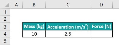
We will determine the product of the two values to obtain the Force value in cell D4.

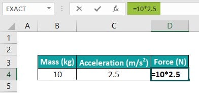
The steps to Write Formula in Excel cell D4 to multiply the two values are,

Step 1: Choose cell D4, and enter the formula=10*2.5

[Alternatively, select cell D4, click, and Write Formula in Excel Formula Bar.

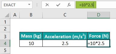
The cursor will remain in the Formula Bar, as shown above.]

Step 2: Press Enter to execute the formula, and view the required product value in the target cell.

The formula multiplies the two specified values to return their product, 25, as shown above.

Method #2 – Using Cell References and Arithmetic Operators

We can supply the cell references to the values while inserting a formula in a cell. And the benefit of using this technique is that if we revise the values in the referred cells, the values get updated in the formula. And it recalculates the new result automatically.

The steps to Write Formulas In Excel using cell references and arithmetic operators are as follows:

1. Choose the cell where we must enter the formula.
2. Enter the ‘=’ symbol. And then, we must click the cells containing the values to insert the corresponding cell references in the formula. Otherwise, we can type the required cell references in excel. And include the applicable operators in the formula to complete the expression.
3. Press Enter to execute the inserted formula in the target cell.

Example #2

Cell C2 in the below image shows the calculation we must perform. And the second table contains the values to use for the evaluation in the target cell E5.

Then, we can use the cell references to the three values and include the applicable arithmetic operators to create the required formula in the target cell. The steps are,

Step 1: Select cell E5, and start typing in the formula with the ‘=’ symbol and ‘(‘, as =(

Step 2: Click cell B5 to select it.

Next, enter the ‘*’ symbol and click cell D5 to choose it.

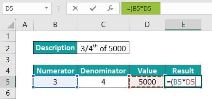
And then, enter the ‘)’, ‘/’, and click cell C5 to enter it in the formula.

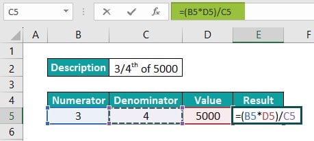
[Alternatively, we can type in the required cell references and the appropriate operators in the required order in cell E5.

Otherwise, choose cell E5, click the Formula Bar, and insert the formula as explained in steps 1 & 2.

Or, as depicted above, we can directly type the formula containing the cell references and the operators in the required order in the Formula Bar.]

Step 3: Press Enter to execute the expression and view the required value in cell E5.

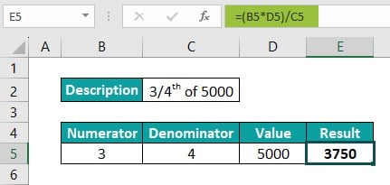
The formula accepts the cell B5 value, 3, and the cell D5 value, 5000. It then multiplies the two values to determine their product, 15000. Next, it accepts the cell C5 value, 4. And finally, it divides the value in the numerator, 15000, with the value in the denominator, 4, to return the value 3750 as 3/4^th of 5000.

Method #3 – Using Defined Names and Arithmetic Operators

We can define names for cells or ranges of cells containing the values required to perform the calculations and use them with the operators to write formulas in Excel.

The steps to Write Formulas in Excel using defined names and arithmetic operators are as follows:

• Select the cell for which we must create a defined name. And enter the required name in the Name Box in excel. [Alternatively, we can select the cell and choose the Define Name option in the Formulas tab or press Alt + M + M + D to open the New Name window. And then, we can enter the required name for the chosen cell in the Name field in the New Name window.

On the other hand, we can select the cell and use the option Name Manager in the Formulas tab or press Ctrl + F3 to open the Name Manager window. And then, when we click New, the New Name window will open, where we can complete the cell name defining process, as explained earlier.]

• Choose the cell where we must enter the formula.
• Enter the ‘=’ symbol. And then, type the first few initial characters of the defined name of the first cell, whose value we must use in the calculation. And Excel will list all the defined names starting with the specified characters. Next, double-click the required defined name to include it in the formula. And include the applicable operators and the remaining defined names to include the corresponding cells in the formula and complete the expression.
• Press Enter to execute the inserted formula in the target cell.

Example #3

The first table contains the inputs required to determine the simple interest value in cell E7. And the target cell’s data format is Currency in Home – Number Format.

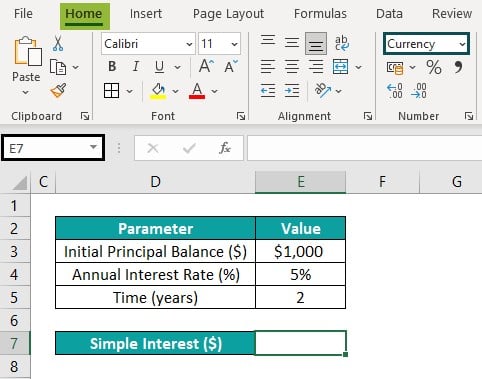
The steps to use the defined names and arithmetic operators for writing a simple interest formula in cell E7 are,

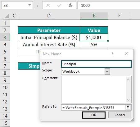
Step 1: Choose cell E3, and enter the term “Principal” in the Name Box to set a defined name for the chosen cell.

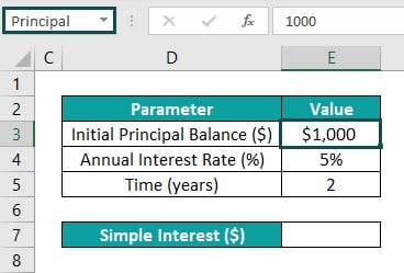
[Alternatively, we can choose cell E3, and select Formulas – Define Name.

The New Name window will open.

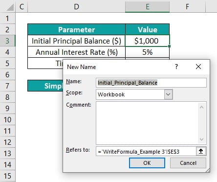
Next, update the name in the Name field to set a defined name for the chosen cell. And click OK.

Otherwise, we can choose Formulas – Name Manager.

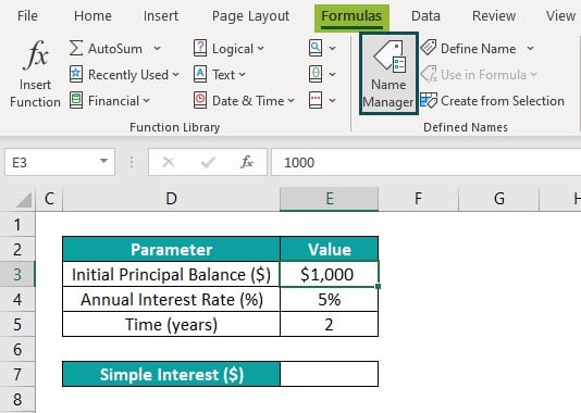
The Name Manager window will open, where we must click the “New” option.

The New Name window will open, as shown below.

And we must update the Name field with the name we need to define for the required cell and the reference to the specific cell in the Refers to field, in the New Name window.

Clicking OK will close the New Name window, and reopen the Name Manager window, where we can view the newly created defined name for cell E3.

Finally, click “Close” to close the window.]

Step 2: Iterate step 1 to define names for cells E4 and E5 as Rate and Time.

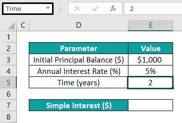
Step 3: Choose cell E7, and enter the ‘=’ symbol. And then, enter the first few characters of the defined name, Principal, set for cell E3.

Excel will list the defined names and inbuilt functions starting with the specified characters. Double-click on the required defined name, Principal, to select it.

Next, enter the arithmetic operator ‘*’. And then, enter the second defined name, Rate, as explained above, to include the cell E4 value in the formula.

And then, enter ‘*’, and the defined name for the cell E5 to complete the formula.

Step 4: Press Enter to execute the formula, and view the required simple interest value, $100, in the target cell.

The cell E7 formula accepts the value in the cell with the defined name Principal, $1,000. Next, it accepts the value in the cell with the defined name Rate, 5%. And then, the formula multiplies the two values to give their product, 50.

Further, the formula accepts the value in the cell the defined name Time references, 2. And finally, it multiplies the previously determined product, 50, by the last input value, 2, to return the required simple interest value as $100.

How To Use Built-In Excel Functions?

In some scenarios, we may be unable to Write Formula in Excel directly. Then, we can use Excel’s built-in functions to build formulas for quickly performing easy to the most cumbersome calculations.

We can use the built-in functions to Write Formula in Excel by following the below methods:

1. Access from the Formulas tab in the Excel ribbon.
2. Enter the function in the Excel cell manually.

Method #1 – Access from The Formulas tab In the Excel ribbon

The steps to insert the required inbuilt function from the Formulas tab are as follows:

1. Choose the cell where we must enter the required formula using the inbuilt function.
2. Select the Formulas tab – Click the Insert Function wizard to open the Insert Function window. Otherwise, we can click the Insert Function icon on the left of the Formula Bar to access the Insert Function window.

Here, we can enter the function description in the Search for a function field if we are unsure about the function name. Otherwise, if we know the function name and the category it belongs to, we can select the category, and choose the function from the list in the Select a function field. And then clicking OK will open the Function Arguments window.

[Alternatively, if we know the function name and the category it belongs to, choose the target cell and select the Formulas tab. We can find a list of function categories in the Function Library group in the Formulas tab, where we can click the required category. And then click the required inbuilt function from the functions listed in the chosen category to open the Function Arguments window.]

• Update the chosen function argument values in the corresponding fields provided in the Function Arguments window.
• Press OK to view the function return value in the target cell.

Example #1 – SUM Function

The table below contains the unit’s sold data for two products.

To determine the total units of the two products sold and display the output in cell F7, we can use the SUM() in the target cell to obtain the required data as follows:

Step 1: Select cell F7, and choose Formulas – Insert Function.

[Alternatively, we can choose cell F7 and click the Insert Function button.

The option is next to the Formula Bar.]

The Insert Function window will open.

Step 2: As the SUM() is a mathematical function in excel,we can select the category Math & Trig.

And then, we can scroll down the functions list to choose SUM().

Next, clicking OK will open the Function Arguments window.

Step 3: With the cursor in the first field in the Function Arguments window, drag the mouse cursor across the cell range F4:I5 to choose the cell range of numbers to add.

And as we do not have further numbers to add, we need not update any argument value in the next field.

Step 4: Click OK to view the SUM() return value, 2494, in the target cell F7.

[Alternatively, choose cell F7, and select Formulas – Math & Trig – SUM function.

The above step will open the Function Arguments window, where we must update the argument value in the first field.

And click OK to execute the SUM(), as explained earlier.]

Method #2 – Enter the Function in the Excel Cell Manually

The steps to insert the required inbuilt function directly into a cell are as follows:

1. Choose the cell where we must enter the required formula using the inbuilt function.
2. Type the ‘=’ symbol, the function name, and ‘(‘. [Alternatively, enter ‘=’, and the first few characters of the function name to choose the required function name from the Excel suggestions by double-clicking it.]
3. Enter the arguments as cell values or references and close the bracket.
4. Press Enter to view the function return value in the target cell.

Please note that we can also enter the inbuilt function in a cell by choosing the target cell, clicking in the Formula Bar, and following steps 2 to 4.

Example #2 – AVERAGE Function

We have the 2021-22 annual sales figures of three branch offices of a firm in two worksheets, 2021_Annual Sales and 2022_Annual Sales, as shown in the below image.

And we must calculate the average annual sales over the two years and display the output in cell D8 in the second worksheet, 2022_Annual Sales. Also, cell D8’s data format is Currency in the Home à Number Format.

Typically, a beginner may be unable to Write Formula In Excel without inbuilt functions in a scenario where the calculations involve multiple sheets.

The steps to manually enter the inbuilt function AVERAGE in the target cell to achieve the desired outcome are as follows:

Step 1: Choose cell D8, and start typing the function =AV, as shown below.

Excel will list the functions starting with the entered characters. And as we require the AVERAGE Excel Function, double-click the function name in the list to select and enter it in the cell.

Next, Excel will show the AVERAGE() syntax, as depicted below, highlighting the argument for which we must provide the value, one at a time.

And then, click the first worksheet tab, 2021_Annual Sales, and select the data range, D3:D5, required for determining the annual average sales.

Next, enter a comma.

And then, click the second worksheet tab, 2022_Annual Sales.

Next, choose the cell range D3:D5, containing the next set of values required to determine the average annual sales figure in cell D8.

Finally, close the bracket.

Step 2: Press Enter to view the AVERAGE() return value, $569,500, as the required average annual sales in 2021-22, in the target cell D8.

[Alternatively, we can choose cell D8, and click on the Formula Bar.

Next, follow the above-mentioned process to enter the inbuilt function in the Formula Bar manually.

The above method will also enter the required formula in the target cell. And pressing Enter will show the AVERAGE() return value in cell D8.]

The cell D8 AVERAGE() accepts two data ranges, one from each sheet. And then, it adds the six values and divides the result by 6 to return the value, $569,500, as the required average annual sales figure.

Important Things To Note

• When we Write Formula in Excel, we must start with the ‘=’ symbol.
• Ensure to use the correct characters as arithmetic operators while using them to enter a formula in a cell manually. Use the characters ‘+’, ‘–‘, ‘*’,’/’, and ‘^’ for addition, subtraction, multiplication, division, and exponent.
• Use the Excel inbuilt functions to create advanced excel formulas required to perform complex calculations involving data in the same and different sheets.

Frequently Asked Questions

Download Template

This article must help understand the Write Formula in Excel, with its formula and examples. You can download the template here to use it instantly.

Recommended Articles

This has been a guide to Write Formula In Excel. Here we create formulas using arithmetic operator, insert inbuilt formulas, examples & downloadable template. You can learn more from the following articles –

• Show Formula In Excel
• Evaluate Formula in Excel
• Excel Subtraction Formula