
What Are Mathematical Functions In Excel?
The Mathematical Functions in Excel have various built-in functions used to calculate numerical data. The commonly used functions are SUM, AVERAGE, COUNT, MIN, MAX, etc.
The Mathematical Functions are categorized under the Math & Trig functions group under the Formula tab.
Use this Mathematical Functions in Excel Template to follow along with the examples in this article.
Download Excel TemplateFor example, we will find the maximum value from the cells having numbers in column A using the Mathematical MAX Excel Function in cell A7 in the following image.
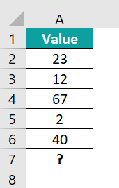
=MAX(A2:A6)
The output comes as ‘67’.
Key Takeaways
- Mathematical functions in Excel are in-built functions used to calculate in Excel.
- The “#VALUE!” error in the SUM function occurs when the text string is over 255 characters long.
- The SUM function automatically ignores empty cells and the cells that contain text.
- The AVERAGE function automatically updates when we include more rows and columns and eliminates when we delete any rows and columns.
- The ROUND function rounds the number per the number of digits allotted in the argument.
- The connected functions to the ROUND function are ROUNDUP and ROUNDDOWN functions.
7 Mathematical Functions Used In MS Excel
#1 – SUM
The SUM excel function enables users to add individual numeric values, cell references, ranges, or all three together using the formula =SUM. Likewise, using the Auto Sum function in Excel, i.e., “∑” automatically adds all the numeric values listed in a particular row or column.
The syntax of the SUM Excel formula is
- number1 = The first numeric value that you want to add. This is the mandatory argument.
- number2 = The second numeric value that you want to add. This is the optional argument.
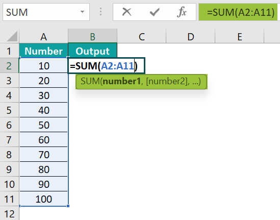
The following example, the image below, depicts a series of numbers 10 to 100. We will sum up the numbers with the Mathematical SUM function.
In the table,
- Column A contains the Number
- Column B contains the Output
The steps to add the given numbers are as follows:
- Step 1: First, we will choose the cell where we want the result to appear. Cell B2 would be the cell in this case.
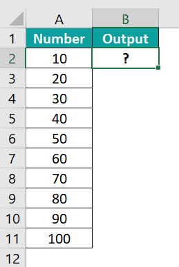
- Step 2: Next, we will enter the SUM formula in cell B2.
- Step 3: Select the array which ranges from the starting cell address to the ending cell address of the table, i.e., A2:A11.
- Step 4: The complete formula entered is =SUM(A2:A11).
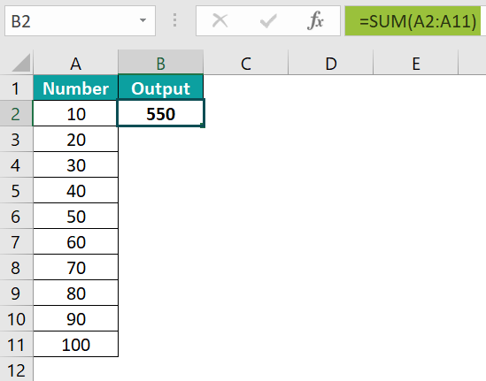
- Step 5: Press the Enter key. The results are shown in cell B2 as 550 in the image below.
#2 – AVERAGE
The AVERAGE Excel function calculates the arithmetic mean of the numbers passed in the arguments. The arguments can be direct numbers or cell references containing numbers.
The syntax of the AVERAGE Excel formula is

- number1 = The first numeric value for which the average is calculated. This is the mandatory argument.
- number2 = The subsequent numeric for which the average is to be calculated. This is the optional argument.
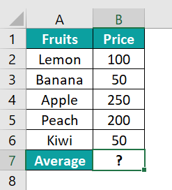
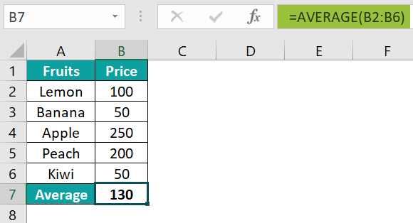
The following example, the image below, depicts the price of fruits. We will try to calculate the average of the numbers with the Mathematical AVERAGE function.
In the table,
- Column A contains the Fruits
- Column B contains the Price
- Cell B7 contains the Output
The steps to calculate the average of the given numbers are as follows:
- Step 1: First, we will choose the cell where we want the result to appear. Cell B7 would be the cell in this case.
- Step 2: Next, we will enter the AVERAGE formula in cell B7.
- Step 3: Select the cell reference from the table, i.e., B2:B6.
- Step 4: The complete formula entered is =AVERAGE(B2:B6)
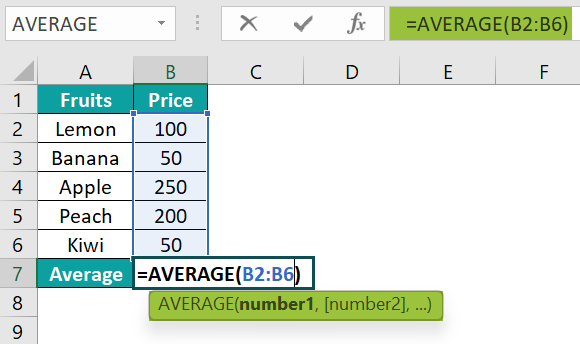
- Step 5: Next, press the Enter key. The result is shown in cell B7 as ‘130’ in the image below.
#3 – AVERAGEIF
The AVERAGEIF Function in Excel returns the arithmetic mean of all numbers in a range of cells based on multiple criteria.
The syntax of the AVERAGEIF Excel formula is
- range=This is the mandatory argument. This is the range to apply the associated criteria against.
- criteria=This is the mandatory argument. These are the criteria to apply against the associated range.
- average_range=This is the optional argument. This is the range of cells that we wish to average.
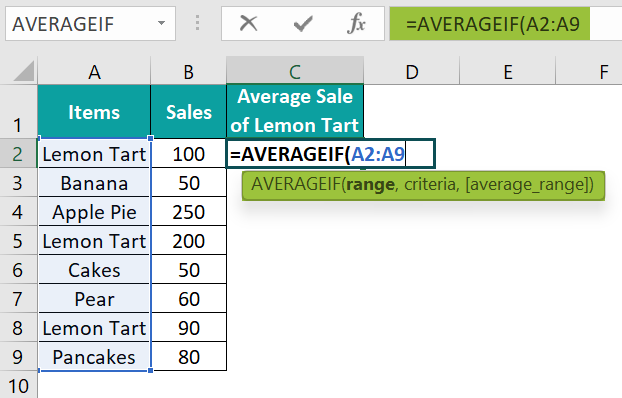
The following example, the image below, depicts items and their sales. We will calculate the average per the criteria for these values using the Mathematical AVEARGEIF function.
In the table,
- Column A shows Items
- Column B contains the Sales
- Cell C2 contains Output
The steps to calculate the average of the given values are as follows:
- Step 1: First, we will choose the cell where we want the result to appear. Cell C2 would be the cell in this case.

- Step 2: Next, we will enter the AVERAGEIF formula in cell C2.
- Step 3: Select the value which ranges from the starting cell address to the ending cell address of the table, i.e., A2:A9.
- Step 4: Set the criteria we want to count, i.e., Lemon Tart.
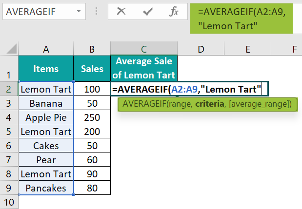
- Step 5: Select the average range, which is the range from the starting cell address to the ending cell address of the table, i.e., B2:B9.
- Step 6: The complete formula entered is =AVERAGEIF(A2:A9, “Lemon Tart,” B2:B9).

- Step 7: Press Enter key. The image below shows the result in cell C2 as ‘130’.
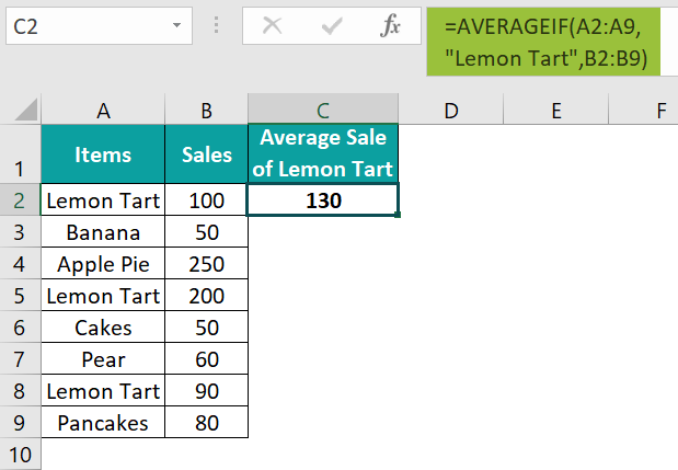
Therefore, the AVERAGEIF function calculates the average per the criteria. In the manual calculation of the average, when the criteria are checked, the value of “Lemon Tart” is as follows;
SUM = 100+200+90 = 390
AVERAGE = {SUM/Number of values}
= 390/3
= 130
#4 – COUNT
The COUNT Excel function calculates the number of cells containing numbers within the given range. The function also counts the number of arguments that have numerical values.
The syntax of the COUNT Excel formula is
- value1 = The first cell reference or the range we want to count. This is the mandatory argument.
- value2 = The second cell reference or the range we want to count. This is the optional argument.
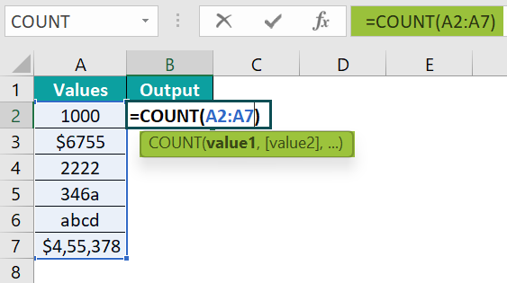
The following example, the image below, depicts values in various formats. We will try counting the cells with numeric values using the Mathematical COUNT formula in cell B2.
In the table,
- Column A shows values
- Cell B2 calculates the number of numeric values
The steps to add the given numbers are as follows:
- Step 1: First, we will choose the cell where we want the result to appear. Cell B2 would be the cell in this case.

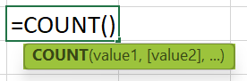
- Step 2: Next, we will enter the COUNT formula in cell B2.
- Step 3: Select the array which ranges from the starting cell address to the ending cell address of the table, i.e., A2:A7.
- Step 4: The complete formula entered is =COUNT(A2:A7).
- Step 5: Press Enter key. The results in cell B2 are as ‘2’ in the image below.
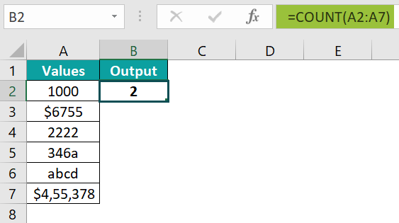
- Therefore, the COUNT function counts only the number as a numerical value, not the number with a variable.
#5 – COUNTIF
The COUNTIF Excel Function counts cells that match specific criteria within the given range.
The syntax of the COUNTIF Excel formula is
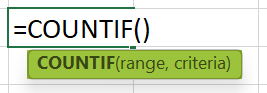
- range=This is a range on which the criteria argument is applied. This is a mandatory argument.
- criteria=This is a condition applied to the range of values argument. This is a mandatory argument.
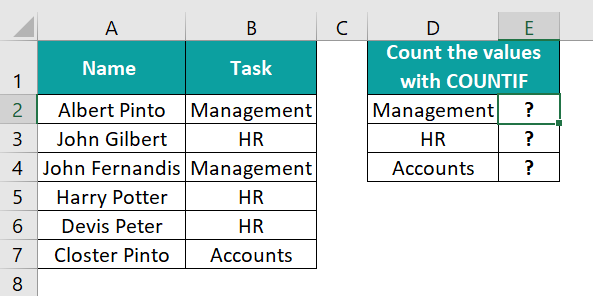
The following example, the image below, shows how the task is assigned to the people. Here, we will try to calculate the number of members in the tasks from the table using the Mathematical COUNTIF function in Excel.
In the table,
- Column A shows the Name
- Column B contains the Task
- Column E contains the Output
The steps to count the number of cells according to the criteria are as follows:
- Step 1: First, we will choose the column where we want the result to appear. Column E would be the column in this case.
- Step 2: Enter the formula that counts the item according to the condition given by the COUNTIF function from the table. Select the range from the starting cell address to the ending cell address of the table, i.e., B2:B7.
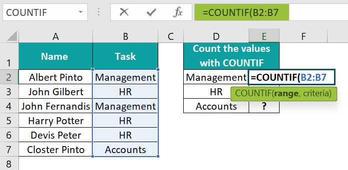
- Step 3: Set the criteria we want to count, i.e., D2, in the below image.
- Step 4: The complete formula is: =COUNTIF(B2:B7,D2).
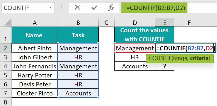
- Step 5: After entering each value in the preceding step, press the “Enter” key. The image below shows the results in cell E2, ‘2.’ The count of the members in the specific task is fetched as output.
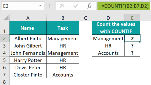
- Step 6: Press Enter key. Drag the formula downwards till cell E4 to get all types of searched results.

Therefore, the COUNTIF function counts the number of task members in the table. The COUNTIF function count as per the criteria given.
#6 – MOD
The MOD excel Function calculates a remainder after dividing a number (dividend) by another number (divisor).
The syntax of the MOD Excel formula is
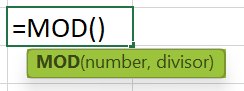
- number = This is the number of which the remainder is calculated.
- divisor = This is the number by which we want to divide the given number.
Unlike other functions, both the arguments of this function are mandatory.
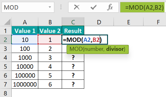
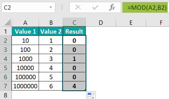
In the following example, the image below depicts the values, and we will calculate the remainder value of the given values using the Mathematical MOD Excel Function.
In the table,
- Column A contains the Value 1.
- Column B contains Value 2.
- Column C contains the Result.
The steps to calculate the value by the MOD Excel Function are as follows:
- Step 1: Select the cell where we will enter the formula and calculate the result. The selected cell, in this case, is cell C2.

- Step 2: Next, we will enter the Formula of the MOD Excel Function in cell C2.
- Step 3: Enter the value of ‘number’ as A2, i.e., the value of the numerator.

- Step 4: Enter the value of the ‘divisor’ as B2, i.e., the value of the divisor.
- Step 5: The entered complete formula is =MOD(A2, B2) in cell C2.
- Step 6: Press Enter key. The results in cell C2 are “0” in the image below.
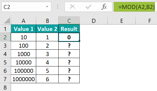
- Step 7: Press Enter key. Drag the formula downwards till cell E4 to get all types of searched results.
#7 – ROUND
The ROUND excel Function rounds up the number to the specified number of digits using the formula =ROUND. It is a part of the Math and Trigonometry function. There are two different functions attached to it: ROUNDUP and ROUNDDOWN. But the ROUND function performs both the tasks round up and round down.
- number = This is the numerical value we want to round up or down. This is the mandatory argument.
- num_digits = This is the number of digits we want to round up. This is also the mandatory argument.
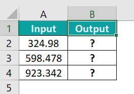
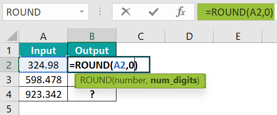
The following example, the image below, depicts the numbers, and we will find the round values using the Mathematical ROUND Excel Function.
In the table,
- Column A contains Inputted numbers
- Column B contains the Output
The steps to round the given numbers are as follows:
- Step 1: First, we will choose the column where we want the result to appear. Column B would be the column in this case.
- Step 2: Next, start by entering the formula in cell B2.
- Step 3: Select the cell that contains the number, i.e., “A2.”
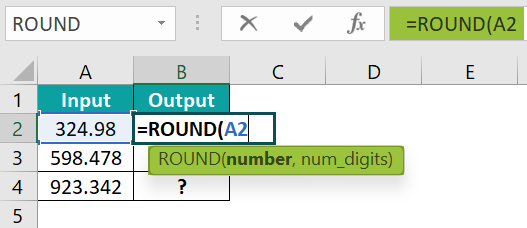
- Step 4: Enter the number of digits to round the values. “0” would be the number digit in this case. This will return the number rounded to 0 decimal places.
- Step 5: The complete formula is: =ROUND(A2,0).
- Step 6: Now, press Enter key. The results are shown in cell B2 as ‘325’ of the image below.
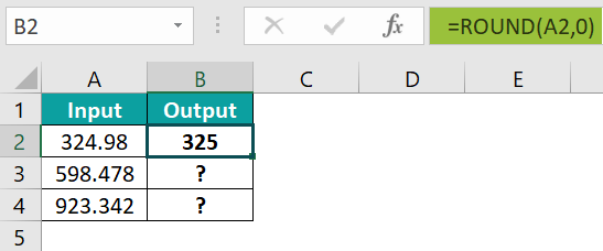
- Step 7: Press Enter key. Drag the formula downwards till cell B4.

Important Things To Note
- The Mathematical functions include ABS, EVEN, ODD, EXP, LN, PI, and more functions in the set.
- The set of Mathematical functions is under the Math & Trig functions in Excel.
- The functions that are part of the Mathematical functions are used to perform mathematical calculations of the given data.
- In business and finance, mathematical functions play a critical role in financial modeling and business valuation methods, where Excel formulas are applied after one or more valuation methods have been selected.
Frequently Asked Questions (FAQs)
The Mathematical function is a rule that gives the value of a variable that depends on specified values of more than one variable. Some functions that are included in the mathematical functions are SUM, MAX, MIN, AVERAGE, etc.
Follow the below steps to insert the Mathematical Functions in Excel; let’s take the MAX function as an example;
• Select the empty cell
• Type =MAX(
• Double-click on the MAX command
• Select the range of the cell or array
• Press Enter.
One can activate the Mathematical function in Excel using the following steps:
1) Choose the empty cell which will contain the result.
2) Go to the Formulas tab and click it.
3) Select Math & Trig from the drop-down menu.
4) Select (any function) from the drop-down menu list.
5) A window called Function Arguments appears.
6) As the number of arguments, enter the values.
7) Select OK.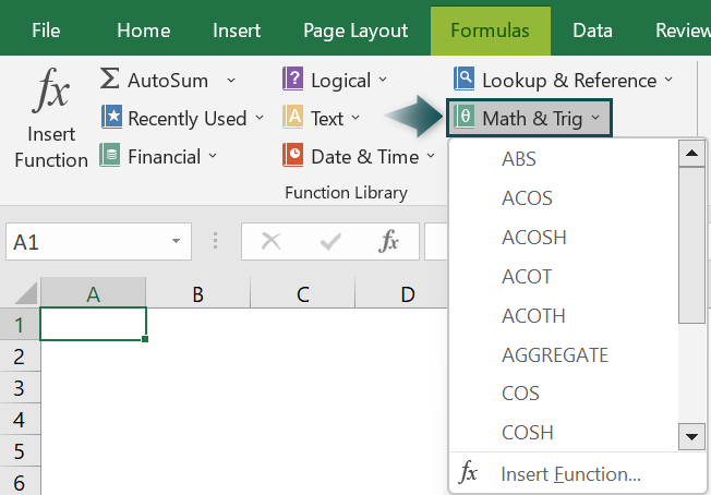
Use this Mathematical Functions in Excel Template to follow along with the examples in this article.
Download Excel Template