
What Is PI In Excel?
The PI in Excel calculates the mathematical value of the function PI, which has the value, 3.141592654. It is the ratio of the circle’s circumference and diameter. It is used to do geometric calculations of the area as new office space, factory, etc.
The PI Excel function is an inbuilt Math & Trig function, so we can insert the formula from the “Function Library” or enter it directly in the worksheet. For example, we will get the PI values using the PI formula for the image below that depicts the Values in column A.

Select cell A2, enter the formula =PI(), and press “Enter”.

The result is ‘3.141592654’ as shown above, i.e., the PI mathematical value.
Use this PI In Excel Template to follow along with the examples in this article.
Download Excel TemplateKey Takeaways
- The PI formula is a Math & Trig function that doesn’t accept any argument but returns its derived value, 3.14159265358979.
- The PI value is the ratio between a circle’s circumference and diameter that is always constant.
- For inserting the PI symbol in Excel, i.e., “π”, open a worksheet, hold the ALT key, and type 227 from the keyboard. So, the shortcut keys are Alt+227.
- We can use the PI() directly to get its value, or enter it in a formula to perform mathematical calculations. We can get accurate results up to 15 digits using the function.
PI() Excel Formula
The syntax of the PI Excel formula is,

There are no arguments for the PI() function.
How To Use PI In Excel?
We can use PI In Excel using 2 ways, namely,
- Access from the Excel ribbon.
- Enter in the worksheet manually.
Method #1 – Access from the Excel ribbon
Choose an empty cell for the output → select the “Formulas” tab → go to the “Function Library” group → click the “Math & Trig” option drop-down → select the “PI” function, as shown below.

The “Function Arguments” window appears. As there are no arguments, just click OK, as shown.

Method #2 – Enter in the worksheet manually
- Select an empty cell for the output.
- Type =PI( in the selected cell. [Alternatively, type =P and double-click the PI Function from the list of suggestions shown by Excel.]
- Press the “Enter” key.
Let us take an example to understand this function.
We will calculate the circle’s circumference of the given circle’s value using PI in Excel.
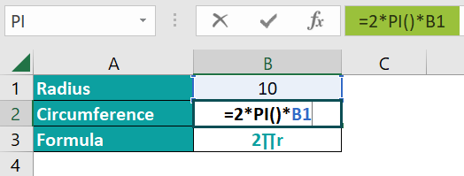
In the table, the data is,
- Row 1 contains the Radius.
- Row 2 contains the Circumference.
- Row 3 contains the Formula of Circumference.

The steps to calculate the value using PI formula are,
- Select cell B2, enter the formula =2PI()B1, i.e., the circle’s circumference is calculated.

- Press the “Enter” key.

The result is “62.83185307” with a circle of 10cm radius, as shown above.

Examples
We will understand some advanced scenarios using the PI in Excel examples.
Example #1
We will calculate the cake’s area of the given values of the cake using the PI function.
In the table, the data,
- Column A contains the Radius of the Cake.
- Column B contains the Area.
- Column C contains the Formula of Area.

The procedure to calculate the value using PI formula is,
Select cell B2, enter the formula =PI()*A2*A2, and press the “Enter” key.

The result is “62.83185307” with a circle of 5cm radius, as shown above.
Example #2
We will calculate the circle’s volume of the given values using the PI function.
In the table, the data is,
- Column A contains the Radius.
- Column B contains the Volume.
- Column C contains the Formula of Volume.

The procedure to calculate the value using PI formula is,
Select cell B2, enter the formula =PI()*4/3*A2*A2*A2, and press the “Enter” key.

The result is “2144.660585” with a circle of 8cm radius, as shown above.
Example #3
We will calculate the sphere’s volume of the given sphere’s values using the PI function.
In the table, the data is,
- Column A contains the Radius.
- Column B contains the Volume.
- Column C contains the Formula of Volume.

The procedure to calculate the value using PI formula is,
Select cell B2, enter the formula =PI()*4/3*A2*A2*A2, and press the “Enter” key.

The result is “33510.32164” with a sphere of 20cm radius, as shown above.
Important Things To Note
- We get the “#NAME?” error if we haven’t typed the brackets, i.e., open and closed parenthesis, for the PI function.
- Since the function doesn’t accept any argument, if we enter a cell value or a cell reference within the brackets, we will get an error message.
- We can calculate any circular object’s values, such as a circle, sphere, round cake, etc., using the PI function.
Frequently Asked Questions (FAQs)
The PI is the ratio between a circle’s circumference and diameter. The PI Function returns the geometric constant value, the symbol of PI is π.
The syntax of the PI formula is =PI()
For example, we will calculate the double value of the PI by multiplying it with 2 of the given values using the PI function.
In the table, the data is,
• Column A contains the Value.
The procedure to calculate the value using PI formula is,
Select cell A2, enter the formula =PI()*2, and press the “Enter” key.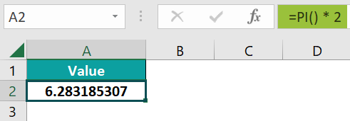
The result is “6.283185307”, as shown above
We can insert the PI Excel Function as follows:
1. Select an empty cell for the output.
2. Type =PI( in the selected cell. [Alternatively, type =P and double-click the PI Function from the list of suggestions shown by Excel.]
3. Press the “Enter” key.
For example, we will calculate the circle’s circumference of the given values using the PI().
In the table, the data is,
• Column A contains the Radius.
• Column B contains the Circumference.
• Column C contains the Formula of Circumference.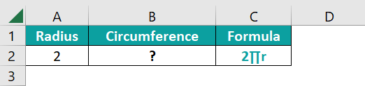
The procedure to calculate the value using PI formula is,
Select cell B2, enter the formula =2*PI()*A2, and press the “Enter” key.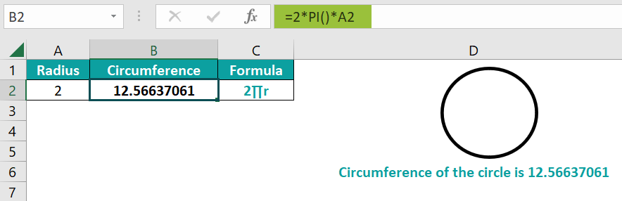
The result is “12.56637061” with a circle of 2cm radius, as shown above.
The PI in Excel is in the “Formulas” tab, as shown below.
Choose an empty cell for the output → select the “Formulas” tab → go to the “Function Library” group → click the “Math & Trig” option drop-down → select the “PI” function, as shown below.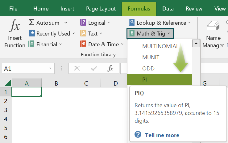
Use this PI In Excel Template to follow along with the examples in this article.
Download Excel Template