MINVERSE In Excel

What Is MINVERSE In Excel?

The MINVERSE in Excel helps users find the inverse of an array or matrix with an equal number of rows and columns. MINVERSE stands for Matrix Inverse. The array input should always be a numeric array.

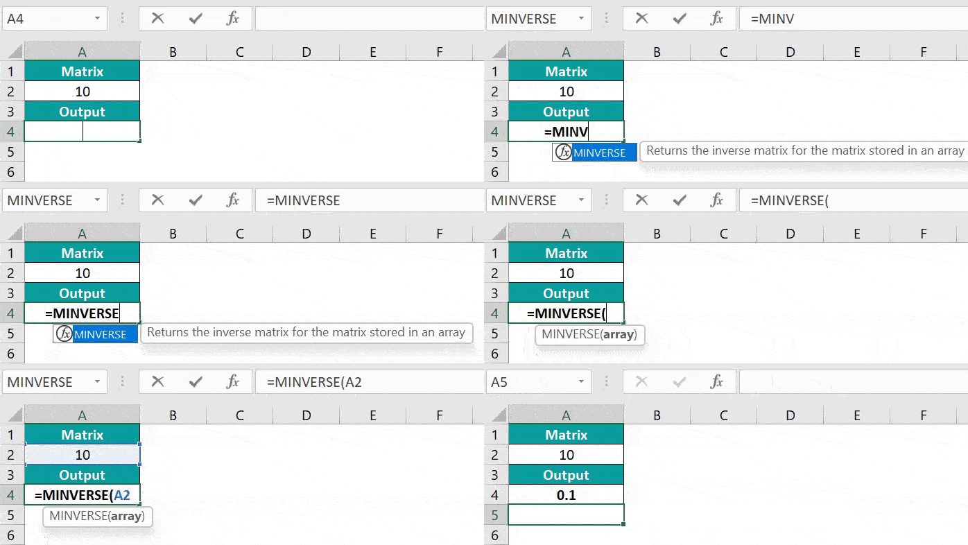
The MINVERSE Excel Function is a built-in function in Excel, so we can insert the formula from the “Function Library” or enter it directly in the worksheet. For example, we will apply the MINVERSE to inverse the matrix of the given values.

Select cell A4, enter the formula =MINVERSE(A2), and press “Enter”. The result is ‘0.1’, as shown below.

What Is MINVERSE In Excel?

MINVERSE Function in Excel is a “Math & Trig” function that inverses the matrix, which is always a square matrix value, i.e., it should have an equal number of rows and columns.
Array arguments can also be provided as array constants such as {2, 3; 4, 5}. Semicolons separate the rows and column arguments within the curly braces.
We must always use the Ctrl+Shift+Enter keys to execute the MINVERSE Function.
The MINVERSE function can accept only one matrix at a time.

MINVERSE() Excel Formula

The syntax of the MINVERSE Excel formula is,

The argument of the MINVERSE Excel formula is,

array: It is a mandatory argument. It specifies an array of values, with an equal number of rows and columns, i.e., 2 rows and 2 columns, 3 rows and 3 columns, and so on…, representing a matrix.

Excel VBA – All in One Courses Bundle (35+ Hours of Video Tutorials)

If you want to learn Excel and VBA professionally, then Excel VBA All in One Courses Bundle (35+ hours) is the perfect solution. Whether you’re a beginner or an experienced user, this bundle covers it all – from Basic Excel to Advanced Excel, Macros, Power Query, and VBA.

Start Learning Now

How to Use MINVERSE Excel Function?

We can use the MINVERSE in Excel using 2 methods, namely,

Access from the Excel ribbon.
Enter in the worksheet manually.

Method #1 – Access from the Excel ribbon

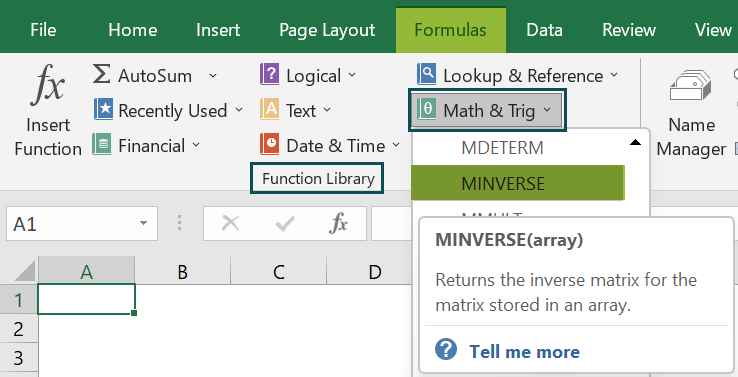
First, choose an empty cell → select the “Formulas” tab → go to the “Function Library” group → click the “Math & Trig” option drop-down → select the “MINVERSE” function, as shown below.

MINVERSE IN Excel - Access from the excel ribbon

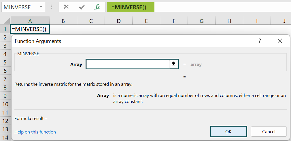
The “Function Arguments” window appears. Enter the argument value in the “Array” field → click “OK”, as shown below.

MINVERSE IN Excel - function arguments window

Method #2 – Enter in the worksheet manually

Select an empty cell for the output.
Type =MINVERSE( in the selected cell. [Alternatively, type =Min and double-click the MINVERSE function from the list of suggestions shown by Excel.
Enter the arguments as cell values or cell references in Excel.
Close the brackets and press “Enter”.

Let us take an example to understand this function.

We will inverse the matrix using MINVERSE in Excel.

In the table, the data is,

Table array A2:C4 contains Value.
Table array E2:G4 contains Output.

The steps to inverse the matrix using MINVERSE in Excel are:

Select empty cells E2:G4, the same number of rows and columns as the input cell range, and enter the formula =MINVERSE(A2:C4).

[ A2:C4 is the array value.]
Press the “Ctrl + Shift + Enter” keys to execute as an array formula.

The results in cells E2:G4 are shown above.

Examples

We will understand some advanced scenarios using the MINVERSE in Excel examples.

Example #1

We will inverse the matrix using the MINVERSE function.

In the table, the data is,

Table array A2:D5 contains Value.
Table array F2:I5 contains Output.

The steps to inverse the matrix using the MINVERSE in Excel function are,

Step 1: Select cells F2:I5 and enter the formula =MINVERSE(A2:D5).

Step 2: Press the “Ctrl + Shift + Enter” keys to execute as an array formula.

The output is shown above.

Example #2

We will inverse the matrix of negative values using the MINVERSE in Excel function.

In the table, the data is,

Table array A2:B3 contains Value.
Table array D2:E3 contains Output.

The steps to inverse the matrix using the MINVERSE function are,

Step 1: Select cells D2:E3, and enter the formula =MINVERSE(A2:B3).

Step 2: Press the “Ctrl + Shift + Enter” keys to execute as an array formula.

The output is shown above.

Example #3

We will inverse the matrix to detect #VALUE! error using the MINVERSE in Excel function.

In the table, the data is,

Table array A2:B3 contains Value.
Table array D2:E3 contains Output.

The steps to inverse the matrix using the MINVERSE function are,

Step 1: Select cells D2:E3, and enter the formula =MINVERSE(A2:B3).

Step 2: Press the “Ctrl + Shift + Enter” keys to execute as an array formula.

The output is shown above.

Example #4

We will inverse the matrix to detect #NUM! error using the MINVERSE in Excel function.

In the table, the data is,

Table array A2:B3 contains Value.
Table array D2 contains Output.

The steps to inverse the matrix using the MINVERSE in Excel function are,

Step 1: Select an empty cell D2, and enter the formula =MINVERSE(A2:B3).

Step 2: Press the “Ctrl + Shift + Enter” keys to execute as an array formula.

The output is shown above.

Important Things to Note

The #NUM! error occurs if the original matrix is zero. Such a matrix is called a Singular Matrix.
The #N/A error occurs if some extra cells are selected under the resulting matrix, which is not a part of the matrix.
The #VALUE! error occurs if there are any blank cell or text values under the given matrix, the matrix should contain numeric values only.

Frequently Asked Questions (FAQs)

1. What does the MINVERSE function do in Excel?

The MINVERSE function reciprocates any square matrix; this process is known as Matrix Inverse. For a matrix to be invertible, there are two basic conditions:

1. The matrix we want to find the inverse needs to be a square matrix which means it should have an equal number of rows and columns.
2. The determinant of the matrix should not be zero. If it is so, the matrix is said to be non-invertible.

The syntax of the MINVERSE in Excel function is =MINVERSE(array).

2. How does the MINVERSE function work in Excel?

We can work with the MINVERSE in Excel function works in Excel as follows:

1.     Select an empty cell for the output.
2.     Type =MINVERSE( in the selected cell. [Alternatively, type =Min and double-click the MINVERSE function from the list of suggestions shown by Excel.
3.     Enter the arguments as cell values or cell references.
4.     Close the brackets and press “Enter”.

For example, we will inverse the following array matrix using the MINVERSE Excel Function.

First select cells A5:B6, enter the formula=MINVERSE(A2:B3), and press the “Ctrl+Shift+Enter” keys.

The results in cells A5 to B6 are shown above.

3. Where is the MINVERSE Function in Excel?

We can find the MINVERSE Function in Excel using the following steps:

First, choose an empty cell → select the “Formulas” tab → go to the “Function Library” group → click the “Math & Trig” option drop-down → select the “MINVERSE” function, as shown below.

Download Template

This article must help understand the MINVERSE Excel Function’s formula and examples. You can download the template here to use it instantly.

MINVERSE In Excel Download

MINVERSE In Excel