
What Is IPMT Function In Excel?
The Interest Payment or the IPMT Excel Function calculates a loan’s periodic interest amount, i.e., the interest portion of the loan amount. The periodic loan payments and the interest are constant. The IPMT Function in Excel is an inbuilt function, so that we can insert the formula from the “Function Library” or enter it directly in the worksheet.
For example, we apply the IPMT Excel Function to evaluate the present value of the loan amount of ‘$20,000’, and the period is “12 years” at ‘10%’ of the interest rate.

Select cell B6, enter the formula =IPMT(B4/12,1,B3*12,-B2), and press the “Enter” key to get the result of $166.67.
Use this IPMT Excel Function Template to follow along with the examples in this article.
Download Excel Template
Key Takeaways
- The IPMT Excel Function is a financial function that calculates the interest amount in a loan where there are constant periodic payments and interest rates.
- Using this function, we can calculate the interest amount for any specific period, such as weekly, monthly, quarterly, semi-annually, or yearly/annually.
- The rate argument of the IPMT function divides the periodic interest rate by the number of periodic loan EMIs.
- Cash paid out is shown as negative numbers, and cash received is shown as positive numbers.
IPMT() Excel Formula
The syntax of the IPMT Excel formula is,

The arguments of the IPMT Excel formula are,
- rate: It is a mandatory argument. It is the interest amount per loan period.
- per: It is a mandatory argument. It is the period to find the interest amount. It must be in the range from 1 to nper.
- nper: It is a mandatory argument. It is the total time period to pay the loan.
- pv: It is a mandatory argument. It is the present amount value.
- fv: It is an optional argument. It is the future amount value to acquire after the last payment. If the fv argument input is not entered, the formula considers it as 0, by default.
- type: It is an optional argument. The type is 0 if the payment is done at the end of the period, and if payments are done or are due at the start of the period, then the type is 1. If omitted, the default value is 0.
How to Use IPMT Excel Function?
We can use the IPMT Excel Function in 2 methods, namely,
- Access from the Excel ribbon.
- Enter in the worksheet manually.
Method #1 – Access from the Excel ribbon
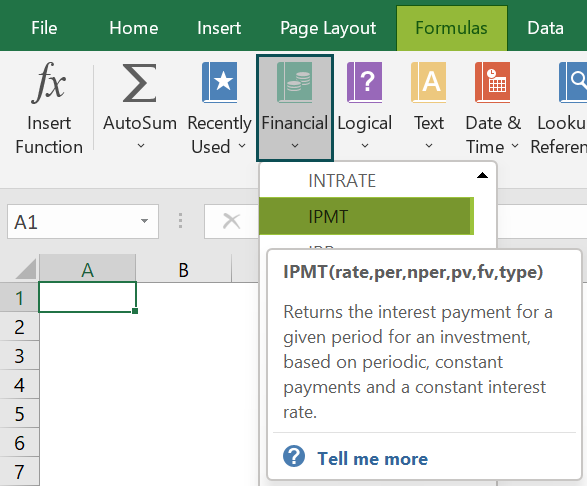
First, choose an empty cell → select the “Formulas” tab → go to the “Functions Library” group → click the “Financial” option drop-down → select the “IPMT” function, as shown below.
The “Function Arguments” window appears. Enter the argument values in the “rate”, “per”, “nper”, “pv”, “fv”, and the “type” fields à click “OK”, as shown below.

Method #2 – Enter in the worksheet manually
- Select an empty cell for the output.
- Type =IPMT( in the selected cell. [Alternatively, type “=I” and double-click the IPMT function from the list of suggestions shown by Excel.]
- Enter the arguments as values or cell references and close the brackets.
- Press the “Enter” key.
Let us take a basic example to understand this function.
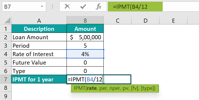
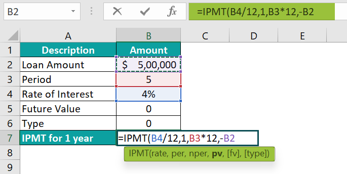
Raj Mohan has taken a loan of $5,00,000 for five years, and the interest rate is 4%. We will calculate his interest amount using IPMT Excel Function.
In the table, the data is,
- Column A contains a Description.
- Column B contains the Amount.

The steps to calculate the semi-annual interest amount using IPMT Excel Function are as follows:
- Select cell B7 and enter the formula =IPMT(B4/12, i.e., the rate of interest value.
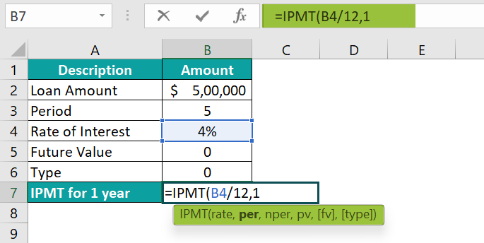
- Put a comma ‘,’, and enter the value of ‘per’ as “1”, i.e., the period value, the formula now is =IPMT(B4/12,1
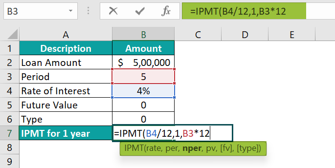
- Put a comma ‘,’, and enter the value of ‘nper’ as “B3*12”, i.e., the total period value, the formula now is =IPMT(B4/12,1,B3*12
- Put a comma ‘,’, and enter the value of ‘pv’ as “-B2”, i.e., the present value, the formula now is =IPMT(B4/12,1,B3*12,-B2
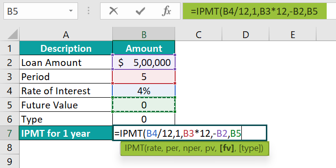
- Put a comma ‘,’, and enter the value of ‘fv’ as “B5”, i.e., the future value, the formula now is =IPMT(B4/12,1,B3*12,-B2,B5
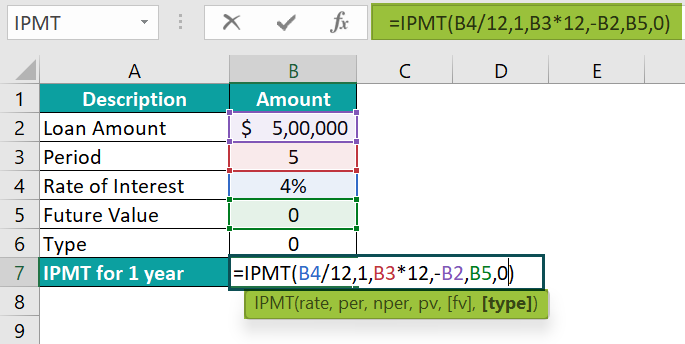
- Put a comma ‘,’, enter the value of ‘type’ as “0”, i.e., the payment type, and close the brackets. The complete formula is =IPMT(B4/12,1,B3*12,-B2,B5,0)
- Press the “Enter” key.
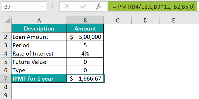
The interest amount is “$1666.67”, as shown in the above image.
Examples
We will understand some advanced scenarios using the IPMT Excel Function examples.
Example #1
Ms. Kathrine has taken a loan of $5,00,000 for five years; the interest rate is 4%. We will calculate the semi-annual interest amount of her investment using the IPMT Excel Function.
In the table, the data is,
- Column A contains a Description.
- Column B contains Amount.

The procedure to calculate the interest amount for the IPMT Function is,
- Select cell B7, enter the formula =IPMT(B4/2,1,B3*2,-B2,B5,0), and press the “Enter” key.
[ ‘rate’ as “B4/2”, ‘per’ as “1”, ‘nper’ as “B3*2” [2 as it is semi-annual], ‘pv’ as “-B2”, ‘fv’ as “B5”, and ‘type’ as “0”]

The interest amount is “$8000.00”, as shown in the above image.
Example #2
Mrs. Lorence has borrowed $80,000 for two years; the interest rate is 15%. We calculate the quarterly interest amount of his investment using the IPMT Excel Function.
In the table, the data is,
- Column A contains a Description.
- Column B contains the Amount.

The procedure to calculate the quarterly interest amount using IPMT Excel Function is,
- Select cell B7, enter the formula =IPMT(B4/4,1,B3*4,-B2,B5,0), and press the “Enter” key.
[‘rate’ as “B4/4”, ‘per’ as “1”, ‘nper’ as “B3*4” [4 as it is quarterly], ‘pv’ as “-B2”, ‘fv’ as “B5”, and ‘type’ as “0”]

The interest amount is “$3,000.00”, as shown above.
Example #3
XYZ company has taken a loan of $25,00,000 for five years; the interest rate is 14%. We will calculate the weekly interest of the company’s investment using the IPMT Excel Function.
In the table, the data is,
- Column A contains a Description.
- Column B contains Amount.

The procedure to calculate the quarterly interest amount using IPMT Excel Function is,
- Select cell B7, enter the formula =IPMT(B4/52,1,B3*52,-B2,B5,0), and press the “Enter” key.
[‘rate’ as “B4/52”, ‘per’ as “1”, ‘nper’ as “B3*52” [52 as it is weekly and 52 weeks in a year], ‘pv’ as “-B2”, ‘fv’ as “B5”, and ‘type’ as “0”]

The weekly interest rate is “$6,730.77”, as shown above.
Important Things to Note
- The nper argument of the IPMT function multiplies the number of years by the number of payments per year.
- The #NUM! error occurs if per value is less than 0 or is less than the value of nper.
- The #VALUE! error occurs when any non-numeric value is entered in the IPMT formula.
- The units must specify the rate and the nper arguments properly. If payment is made monthly, as on a 4-year loan at 24% annual interest, we need to use 24%/12 for rate and 4*24 for nper, and if the annual payments are made on the same loan, use 24% for rate and 4 for nper.
Frequently Asked Questions (FAQs)
The IPMT function calculates the interest part based on a given loan amount and the payment time. The interest payment for the first, last, or any period in between is evaluated using the function.
The IPMT Excel Function is categorized under the Excel Financial functions of the Functional Library.
The syntax of the IPMT function is =IPMT(rate,per,nper,pv,[fv],[type])
We can work with the IPMT Excel function as follows:
1. Select an empty cell for the output.
2. Type =IPMT( in the selected cell. [Alternatively, type “=I” and double-click the IPMT function from the list of suggestions shown by Excel.]
3. Enter the arguments as values or cell references and close the brackets.
4. Press the “Enter” key.
For example, we apply the IPMT Excel function to evaluate the present value of the loan amount of ‘$1,00,000’, and the period is “5 years” at ‘3%’ of the interest rate.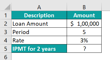
Select cell B6, enter the formula =IPMT(B5/12,1,B4*12,-B2), and press the “Enter” key.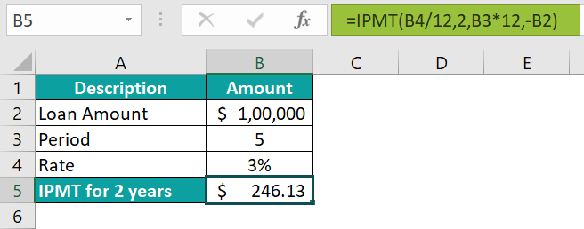
The result is ‘$246.13’, as shown above.
The IPMT Excel Function is in the “Formulas” tab and can be inserted as follows:
First, choose an empty cell → select the “Formulas” tab → go to the “Functions Library” group → click the “Financial” option drop-down → select the “IPMT” function, as shown below.
Use this IPMT Excel Function Template to follow along with the examples in this article.
Download Excel TemplateRecommended Articles
Continue with these related resources when you want the next practical step in this topic.
Explore the full Excel Financial Functions guide or browse Excel Resources.