
What Is Excel Statistics?
Statistics in Excel is a way to perform statistical studies involving the collection, organization, evaluation, interpretation, and presentation of empirical data. The software offers Statistical functions and practical analysis tools for statistical calculations and reviews.
Users can use Excel statistics as a quantitative tool to conduct statistical analysis of massive datasets in domains such as business, marketing, engineering, and health.
Use this Statistics In Excel Template to follow along with the examples in this article.
Download Excel TemplateFor example, the table below contains a set of scores out of 100.

If the requirement is to analyze the descriptive statistics in Excel for the above data. Then, we can use the Data Analysis ToolPak feature in the Data tab to conduct the required statistics in Excel analysis.

Here is how to interpret the obtained data for Descriptive Statistics in Excel.
The Mean, 82.57,is the average of the given data, and the Standard Error, 3.146, gives the accuracy with which the sample distribution denotes the population. And higher its value, the more will be variability.
On the other hand, the Median gives the middle value in the sorted scores. And Mode shows the value that appears the maximum number of times in the dataset. In our case, both the values are the same, 85.
And while the Standard Deviation, 11.77,measures the standard deviation for the given data, the Sample Variance, 138.57,is the square of the Standard Deviation.
Next, the Kurtosis, -0.99, indicates the deviation of the tails of the distribution from the tails of the normal distribution. And the Skewness, -0.186, denotes the asymmetry of the given data.
Furthermore, the Range, 37, gives the difference between the maximum and minimum values in the dataset.
And the Minimum and Maximum (63 and 100) give the least and highest values in the given dataset. And the Sum and Count (1156 and 14) represent the total of all the data points in the dataset and the total number of data points.
Thus, with the above parameters, we can obtain the summary statistics in Excel in just one go, making Excel a very useful tool for conducting statistical studies quickly.
Key Takeaways
- Statistics in Excel enables one to collect, arrange, interpret and present data for conducting statistical studies.
- Users can use the Excel functionality to perform statistical reviews of marketing, business, engineering, and health-related datasets.
- Excel offers inbuilt Statistical functions such as AVERAGE, COUNT, MIN, MEDIAN, MAX, and MODE to perform basic statistical data calculations and analysis.
- Excel provides tools such as ANOVA, Descriptive Statistics, T-Test, Regression, and Z-Test for advanced statistical data calculations and reviews. And one can access them using the Data Analysis ToolPak feature in the Data tab.
How To Use Excel Statistical Functions?
We shall see how to use the different functions to calculate statistics in Excel.
#1 – Find Average Sale Per Month
Typically, businesses monitor their firm’s average sales figures to make critical decisions. And data such as the average monthly sales, expenses, and profit values provide deep insights into their business performance.
For example, the table below contains a company’s average monthly sales, expenses, and profit figures.

We can perform the basic statistics in Excel analysis using the AVERAGE Statistical function in the target cell range D14:F14, as shown below:
- Step 1: Select the target cell D14, enter the AVERAGE excel function, and press Enter.
=AVERAGE(D2:D13)

[Alternatively, select the target cell D14 and follow the path Formulas → More Functions → Statistical → AVERAGE to open the Function Arguments window.


We shall enter the sales data range as the Number1 field value in the Function Arguments window.

And clicking OK will give the average sales value in cell D14.]
- Step 2: Drag the excel fill handle to the right till cell F14 to update the formula in cells in the range E14:F14.

Thus, the results show that the average monthly sales of $31,210.69 exceed the expenses of $27,263.56. And so, the average monthly profit is a positive value, $3,947.13, indicating the average monthly business performance is good.
#2 – Find Cumulative Total
Reviewing the cumulative total of business facets, such as monthly or yearly sales figures and order data, is another way of performing the basic statistics in Excel analysis.
For example, the table below contains a firm’s yearly order data in column D from 2017-2022.

And the requirement is to determine the cumulative total orders from 2017-2022 in column E to analyze the years when the total orders increase was relatively less.
Then, we can use the SUM excel function in the target cells to calculate statistics in Excel and perform the required analysis.
- Step 1: Select the target cell E2, enter the SUM(), and press Enter.
=SUM($D$2:D2)

- Step 2: Using the fill handle, enter the formula in cell range E3:E7.

The cells in the range E3:E6 show error as there are adjacent cells which we do not consider while finding the required cumulative total. So, we can ignore the errors. And for that, click cell E3 and then the error warning icon.

Next, choose the Ignore Error option from the list.

Likewise, ignore the errors in the remaining cells to get the below output.

Thus, we can determine when the firm witnessed a slower increase in the total order count from the cumulative total data.
#3 – Find Percentage Share
Every business tracks its achieved annual revenue targets. However, the revenue share does not remain the same every month. While the business makes more revenue in certain months, the figures may plunge in other months.
Thus, we can find the monthly percentage share to calculate the statistics in Excel and analyze in which months the revenue was relatively higher.
For example, the table below shows a company’s monthly revenue.

Here is how to find the percentage share of revenue each month, assuming cells in the range F2:F13 are the target cells.
- Step 1: Select cell E14, enter the SUM() to find the company’s total revenue, and press Enter.
=SUM(E2:E13)

We find the total revenue as we require the value to determine the monthly revenue share in column F.
- Step 2: Select the target cell F2 with the data format in Home → Number Format set as Percentage, and enter the below formula to find the percentage revenue share for January.
=E2/$E$14

The expression uses the absolute reference to the cell containing the total revenue, as the value must remain constant while finding every month’s percentage revenue share.
- Step 3: Using the fill handle, enter the formula in cell range F3:F13.

Thus, we can infer from column F data that October and April had the highest contributions to the firm’s overall revenue, 11.75% and 11.03%. And on the other hand, the month with the least contribution to the firm’s overall revenue was July, with a percentage share of 4.69%.
#4 – ANOVA Test
We saw an illustration explaining the summary statistics in Excel analysis using the Data Analysis ToolPak feature in the Data tab in the What is Excel Statistics? Section.
But the feature also includes another option to perform statistical analysis in Excel, the Anova: Single Factor test. It helps determine the best alternative from the given options.
For example, we have three products tested for different grades, with the test results in mg and a higher mg value being the preference.

Then, here is how to use the Anova: Single Factor test and determine whether the test results of the three products are similar or significantly different. And hence, find the best product among the three.
But first, we must check if the Data tab shows the Data Analysis option.

And if the Data tab does not display the Data Analysis option, as shown in the above image. Then the steps to install it are as follows:
- Step 1: Click File → Options to open the Excel Options window.


- Step 2: Choose Add-ins and click Go in the Excel Options window.

- Step 3: The Excel Add-ins window opens, where we must click the Analysis ToolPak box and press the OK button.

Once we click OK, the Data tab will display the Data Analysis option, as shown below.

- Step 4: Select Data → Data Analysis to open the Data Analysis window.

- Step 5: Choose the Anova: Single Factor option from the Analysis Tools list in the Data Analysis window.

And clicking OK will open the Anova: Single Factor window.

- Step 6: Update the Input Range as the cells containing the three products’ data. And as the given data is in columns, the Grouped By option should be Columns. Also, we will check the labels option box as the chosen input range includes the column headings, and we require the test result to display the column headings.
On the other hand, the Alpha, by default, is 0.05. And we will not change it.
Finally, we will update the Output Range to display the output in a cell in the current worksheet, as shown below.

- Step 7: Click OK to obtain the below result.

The F value, 1.259, is less that the F crit, 5.143. Also, the P-value is 0.349, more than the significant threshold (Alpha) of 0.05.
Thus, the inference is that we cannot reject the null hypothesis that there is no considerable difference between the three products’ results.
And the averages of the three products being more or less the same corroborates our findings. Thus, choosing any one of them will give a similar experience.
Important Things To Note
- If we cannot find the Data Analysis option in the Data tab to access the Data Analysis ToolPak feature to perform the statistics in Excel calculations and analysis, then, we need to install the Analysis ToolPak add-in from Excel Options under the File tab.
- Use the Descriptive Statistics option in the Data Analysis ToolPak feature to perform summary statistics analysis in your worksheet.
Frequently Asked Questions (FAQs)
The use of Excel in statistics is that it makes data collection, organization, and manipulation in rows and columns before commencing with the statistical analysis convenient and quick.
The statistical tools used in Excel are the options we can access using the Data Analysis ToolPak feature in the Data tab. And some of the prominent statistical tools are:
• ANOVA Test
• Descriptive Statistics
• Regression
• F-Test
• T-Test
• Z-Test
We can calculate frequency in statistics Excel using the Statistical function FREQUENCY.
For example, the first table contains the height values of ten candidates.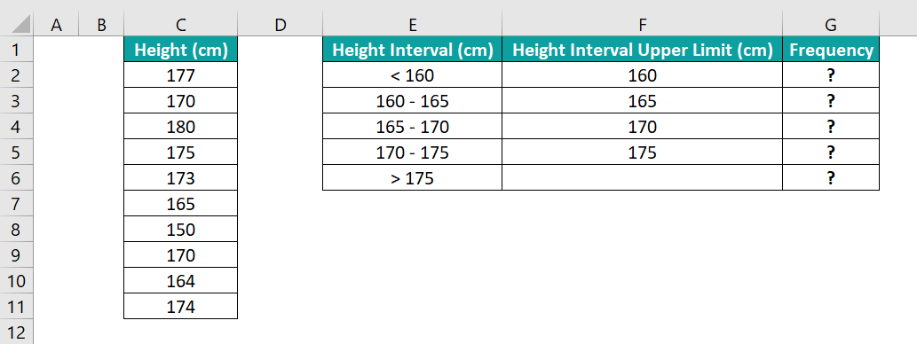
And the requirement is to determine the number of candidates in each height interval specified in the second table and display the results in cells G2:G6. Also, column F shows the upper limit of each height interval.
Then, we can apply the Statistical function FREQUENCY as an array formula in the target cells and achieve the required data.
• Step 1: Select the cell range G2:G6.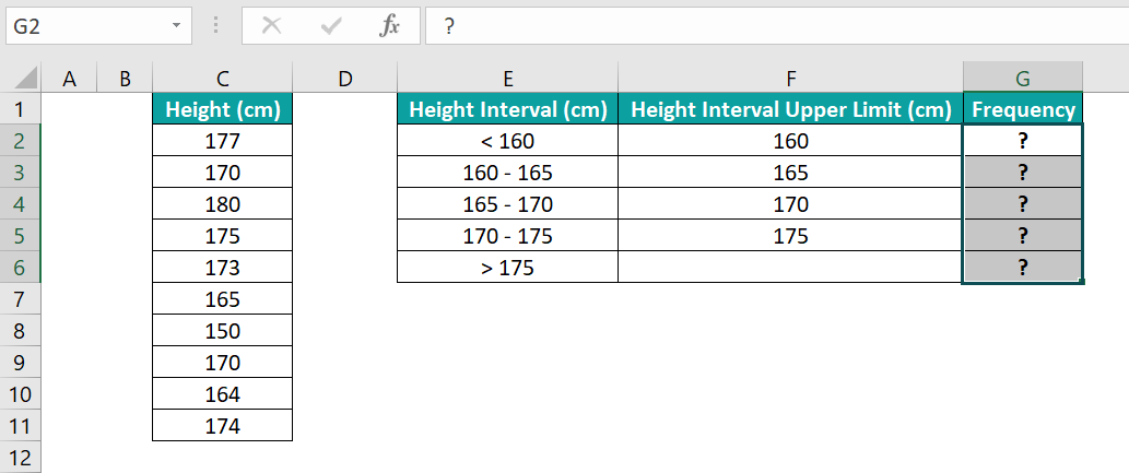
• Step 2: Enter the FREQUENCY() as shown below.
=FREQUENCY(C2:C11,F2:F5)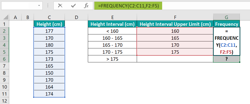
• Step 3: And press Ctrl + Shift + Enter to execute the FREQUENCY function as an array formula.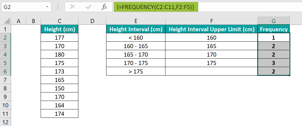
Let us check cell G6 to understand how the formula works. The formula checks cells C2:C11 for values greater than 175 cm. And as cells C2 and C4 contain height values 177 cm and 180 cm, greater than 175 cm, the formula returns the frequency as 2.
Use this Statistics In Excel Template to follow along with the examples in this article.
Download Excel Template