
What Is AVERAGEIF Function In Excel?
The AVERAGEIF function in Excel determines the average/mean of the selected cells in a dataset that satisfies the required criteria. The function is used to evaluate the central tendency, a measure representing the center of a set of data values in a statistical distribution.
The AVERAGEIF Excel function is an inbuilt Statistical function, so we can insert the formula from the “Function Library” or enter it directly in the worksheet.
Use this AVERAGEIF Function in Excel Template to follow along with the examples in this article.
Download Excel TemplateFor example, the first table below contains a list of fruits and their quantity, and the second table shows the criterion to determine the quantity values provided in the first table to get the average.

We will use the Excel AVERAGEIF function to calculate the average. Select cell F6, enter the formula =AVERAGEIF(B2:B7,F3), and press “Enter.”

The output is shown above. The function averages the values in the given data range B2:B7, which are greater than 0. Thus, the result, 450 pounds, is the average of the quantities 500, 450, 550, and 300.
Key Takeaways
- The AVERAGEIF function in excel evaluates the average of the cell values in a supplied range that fulfill the given conditional criteria.
- The AVERAGEIF() accepts two mandatory arguments, range and criteria, and one optional argument, average_range, as input. The range can include numbers, names, arrays, or cell references to numbers. And the criteria can be number, text, expression, or cell reference.
- The AVERAGEIF() allows wildcard characters, ‘?’ and ‘*’, in the criteria argument to match a single character or sequence of characters, respectively.
AVERAGEIF() Excel Formula
The syntax of the Excel AVERAGEIF formula is:

The arguments of the Excel AVERAGEIF formula are:
- range: The cell range of a dataset to test against the specified criteria. It is a mandatory argument.
- criteria: The criteria to check the specified cells to average. It is a mandatory argument.
- average_range: The actual range of cells that we require to average. It is an optional argument.
How To Use AVERAGEIF Excel Function?
We can use the AVERAGEIF excel function in 2 methods, namely,
- Access from the Excel ribbon.
- Enter in the worksheet manually.
Method #1 – Access from the Excel ribbon
First, choose an empty cell for the output → select the “Formulas” tab → go to the “Function Library” group → click the “More Functions” option drop-down → click the “Statistical” option right arrow → select the “AVERAGEIF” function, as shown below.

The “Function Argument” window appears. Enter the argument values in the “Range, Criteria, and Average_range” fields → click “OK”, as shown below.

Method #2 – Enter in the worksheet manually
First, ensure the given range is not empty/blank and does not include only text values.
- Select the target cell for the output.
- Type =AVERAGEIF( in the cell. [Alternatively, type =A or =AV and double-click the AVERAGEIF function from the Excel suggestions.]
- Enter the arguments as cell values or cell references in Excel.
- Close the brackets and press Enter to execute the function.
Let us take an example to understand this function.
We will find the state-wise average household income for the state specified using Excel AVERAGEIF function.
The table below lists the top ten richest US cities, their states, and the respective average household income details.
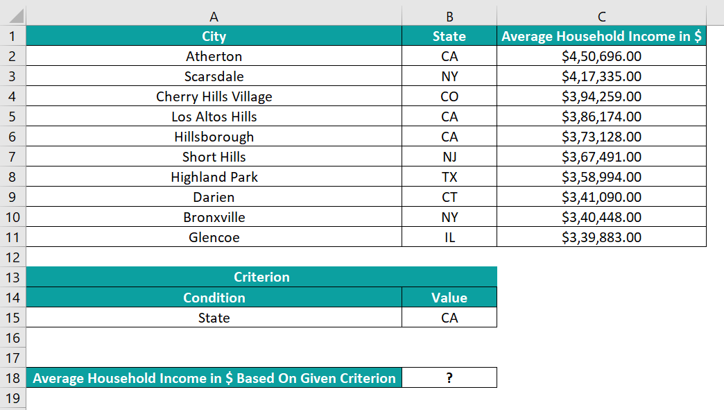
The steps to find the average using AVERAGEIF function in Excel are,
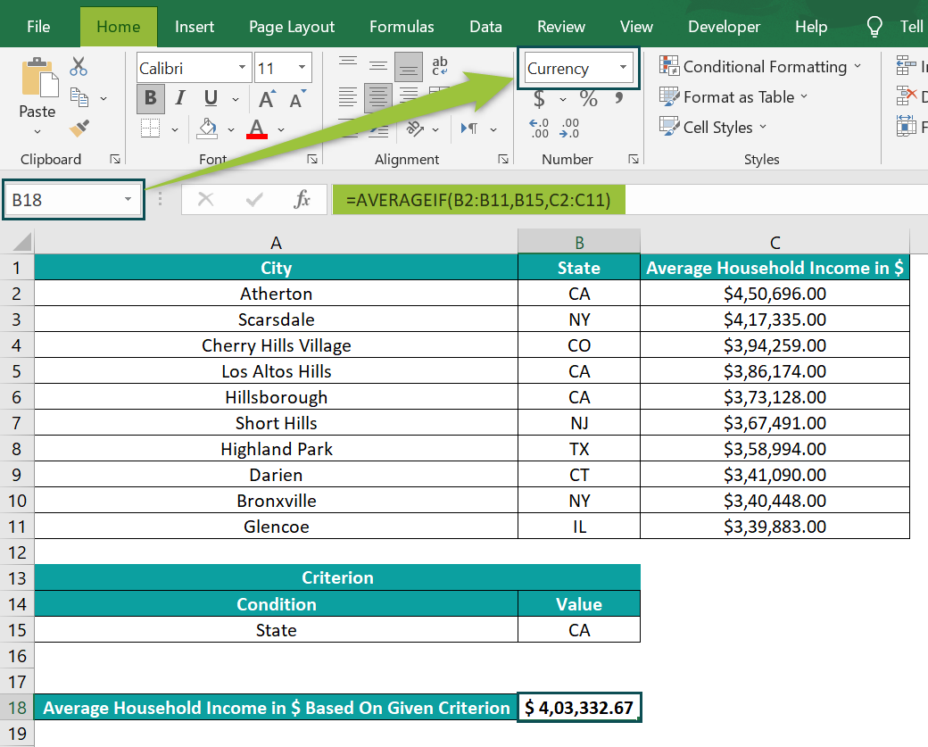
- Select cell B18, enter the formula =AVERAGEIF(B2:B11,B15,C2:C11), and press Enter.
[Also, enter the formula as =AVERAGEIF(B2:B11,”CA“,C2:C11), cell value instead of a cell reference.]
- Select cell B18 and set the Number Format in the Home tab as Currency to view the required average household income in the state of CA as a currency value.

The output is shown above. First, the function checks the cell range B2:B11 for the state name, “CA”, and finds three instances in cells A2, A5, and A6. Then considers the corresponding cell values from the cell range C2:C11 and returns the average value as $403,332.67.
[Alternatively, we can apply the AVERAGEIF() as follows: click Formulas → More Functions → Statistical → AVERAGEIF, which will open the Function Arguments window.
Then, enter the respective AVERAGEIF() arguments in the Function Arguments window.
And finally, click OK in the Function Arguments window to execute the function.]


Examples
We will understand some advanced scenarios using the Excel AVERAGEIF function examples.
Example #1
We can use the wildcard characters, ‘?’ or ‘*’, in the criteria argument, when the given criterion involves a partial match and apply the AVERAGEIF Excel function.
The first table in the image below contains a list of inventory items and their quantity details.

The procedure to find the average number of boxes of all oil varieties using the AVERAGEIF function in Excel is,
Select cell E6, enter the formula =AVERAGEIF(A2:A12,E3,B2:B12), and press Enter.

The output is shown above.
[Output Observation: The wildcard character asterisk, ‘*’, helps match a sequence of characters. So, when we use it in the AVERAGEIF(), the function tries to find a partial match for the phrase “oil” in the given cell range, A2:A12. And it gets the required matches in cells A2, A5, A7, A11, and A12.
Then, it calculates the average of the corresponding column B cell values, 200, 250, 100, 100, and 50, in cells B2, B5, B7, B11, and B12, and returns the average number of boxes of all oil varieties, 140.]
Example #2
Let us see how the Excel AVERAGEIF function works if the range of values to find the average includes blank and non-blank cells.
The below table contains a list of students, their scores, and scholarship details.

The procedure to determine the average using the Excel AVERAGEIF function is,
Select cell B18, enter the formula =AVERAGEIF(B2:B11, “<>”,C2:C11), and press Enter.

The output is shown above.
[Output Observation: The above AVERAGEIF() checks for non-empty cells in column B as the students with a scholarship have the scholarship status as Yes in column B. Here the criteria argument includes ‘<>’ to check for non-empty cells, B3, B4, B6, B9, and B11.
And then, the function averages the scores in the corresponding column C cells (C3, C4, C6, C9, and C11), 495, 478, 453, 486, and 470, to return the average total score as 476.4.]
Example #3
We will use the Excel AVERAGEIF function for multiple criteria.
The following table shows a list of participants from different states and their respective timing details during a competition. It shows more than one participant belonging to the same state, such as GA and NY.

The procedure to use the Excel AVERAGEIF function for multiple criteria is:
Select cell G7, enter the formula =AVERAGE(AVERAGEIF(B2:B16,G3,C2:C16),AVERAGEIF(B2:B16,G4,C2:C16)), and press Enter.

The output is shown above.
[Output Observation: The above formula determines the average time taken by participants from the states, GA and NY, separately. And then, find the average of the two average values the Excel AVERAGEIF function returns.
So, the first AVERAGEIF() checks for the participants from GA and then averages the corresponding time values, 77, 63, 70, and 73, to return the value of 70.75 seconds. Next, the second AVERAGEIF() checks for the participants from NY and then averages the corresponding time values, 80, 61, and 50, to return the value of 63.66 seconds. And finally, the AVERAGE() returns the average of the values 70.75 and 63.66, 67.20833 seconds.]
Important Things to Note
- If no cells in the supplied range satisfy the specified criteria, or an empty range is selected, or a range with only text values, then we get the #DIV/0 error.
- If the criteria argument contains an empty cell, the function assumes it as 0.
- The AVERAGEIF() ignores cells containing logical values, TRUE or FALSE, in the given range. And the function also ignores empty cells in average_range.
- If we ignore the argument average_range, the function uses the given range.
Frequently Asked Questions (FAQs)
There is an AVERAGEIF function in Excel. It is in the Formulas tab, and we can select Formulas → More Functions → Statistical → AVERAGEIF to apply it in the required cell.
We can use AVERAGEIF() with the date criterion in Excel if we need the average units dispatched after 4/1/2022.
For example, the following table contains a list of items and their dispatch details.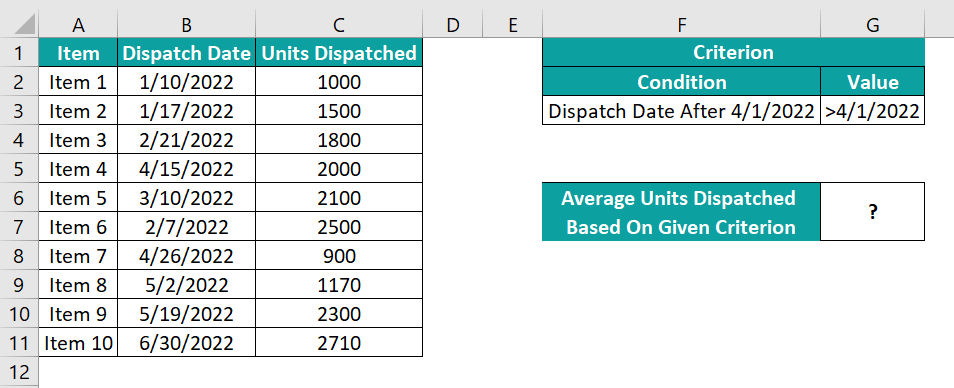
The procedure to apply the Excel AVERAGEIF function with the required date criterion is:
Select cell G6, enter the formula =AVERAGEIF(B2:B11,G3,C2:C11), and press Enter.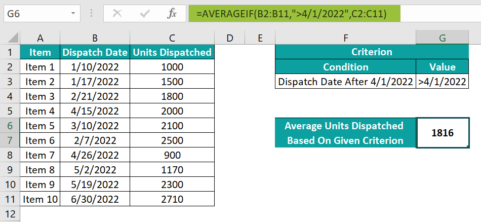
The above formula checks for dates after 4/1/2022 in column B and then determines the average of the corresponding units, 2000, 900, 1170, 2300, and 2710, 1816 units.
We can use the AVERAGEIF() in Excel with a logical operator in the criteria and determine the average contribution by volunteers aged 25 and above.
For example, the below table contains the details of the contributions made by a set of volunteers.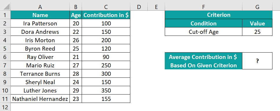
The procedure to apply the AVERAGEIF Excel function by volunteers aged 25 and above is,
Select cell G6, enter the formula =AVERAGEIF(B2:B11,”>=”&G3,C2:C11), and press Enter.
[Note: However, we may also enter the formula as =AVERAGEIF(B2:B11,”>=25″,C2:C11)]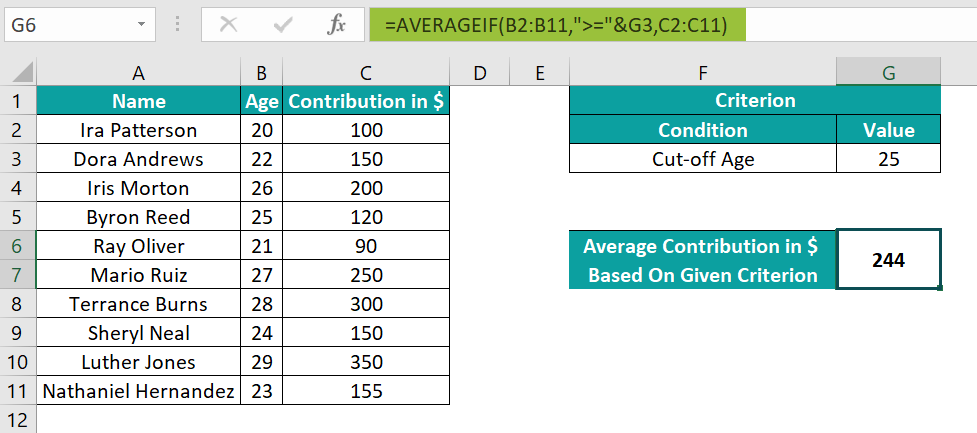
The output is shown above.
[Output Observation: In this case, we must provide the required logical operator and the number in double quotations when supplying them as the criteria argument.
In the above formulas, the function checks for cells containing ages 25 and above in column B. And then, it averages the corresponding contribution values in column C (200, 120, 250, 300, and 350) to return the value of $244.]
Use this AVERAGEIF Function in Excel Template to follow along with the examples in this article.
Download Excel Template