What Is CAGR Formula in Google Sheets?
CAGR is the compound annual growth rate, which shows us the annualized average revenue growth rate between any two years (e.g., 2015 and 2021). The CAGR can be calculated for an investment over a period of year. It shows the average revenue growth in a particular period. In simple terms, it helps you understand how much you have earned in an investment over a period of time.
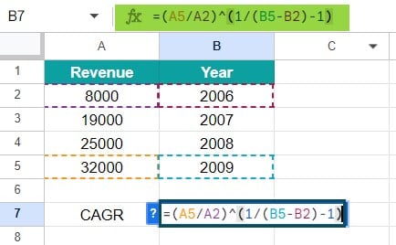
It is essential to understand that CAGR is different from the general growth rate as it is repetitive. General growth rates may vary from year to year. There is no direct CAGR formula in Google sheets to calculate this value. Instead, you can use the formula below. Below are the company’s financial details. To find a single number that shows the growth rate over four years, you can use the compound annual growth rate formula.
📥Download the ready-to-use Excel template to practice this tutorial yourself.
CAGR Formula in Google Sheets
In general, it is used in financial analysis and by business owners to find the growth of their business or compare their revenue with competitors.
Table of Contents
Key Takeaways
- CAGR stands for compound annual growth rate, and it tells is the average annualized growth rate in revenue during a particular time period.
- The formula to calculate the CAGR is as follows: CAGR = (future value / present value)1/periods – 1.
- Besides the above formula, we use functions such as POWER, RATE and IRR to calculate the CAGR value. Of these, IRR is the most straightforward method.
- Analysts use the compounded annual growth rate to calculate the average growth of an investment. It can also be helpful in comparing investments of different types.
Calculating the CAGR formula in Google Sheets is simple and can be done using any of the ways mentioned above. Google Sheets may introduce a direct CAGR function, which could make the calculations even more accessible.
CAGR Standard Formula Syntax
CAGR = EV / SV ^ (1/n) – 1
- EV – Refers to the end value
- SV – Refers to the start value
- n – Represents the number of years
How to Use CAGR Formula in Google Sheets?
Let us look at the different ways in which we can use the CAGR formula in Google Sheets to find the revenue growth in a particular time period and compare it with competitors.
#1 – Basic Method
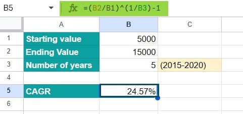
Let’s look at the primary method of applying the CAGR formula to compute CAGR. We have to calculate the CAGR for the period from 2015 to 2020. So, we use the formula CAGR = EV / SV ^ (1/n) – 1 here. Let us tabulate the required starting and ending values and the number of years in a Google sheet, as shown below.

Step 1: Apply the following formula in call B5.
=(B2/B1)^(1/B3)-1

Step 2: Press Enter. You get 0.24573 or 24.57% as the CAGR value. It represents the compound annual growth rate of the investment during these five years.

Step 3: We can confirm the answer by applying the CAGR percentage and finding the end value.
#2 – Using the Power Function
There is no one way or direct formula to calculate the CAGR in Google sheets. You can follow a multitude of formulas and functions. Another way to calculate the CAGR is to use the POWER function in Google Sheets. Let us see how!
As seen in the previous example, the formula to calculate the CAGR value is
CAGR = EV / SV ^ (1/n) – 1
Instead of using the ^ symbol each time, we can easily apply the POWER function. Consider the details below entered in a Google sheet.

Step 2: Apply the following function in cell B5.
=POWER(B2/B1, 1/B3)-1
This is derived from the formula =POWER (Ending Value/Beginning Value, 1/n)-1
Here, the POWER function replaces the ˆ used in the previous example’s formula. Press Enter.


As observed, a value of 0.605 or 6.05% is calculated as the CAGR.
#3 – Using the RATE Function
Another method for calculating CAGR is using the RATE function. We use this function to return the interest rate per period of an annuity investment based on constant amount periodic payments. The formula is as follows:
RATE(nper, pymt, present_value, [future_value, end_or_beginning, guess])
Let us look at the arguments a little more in detail.
- Nper – the total number of payments for the annuity, i.e., the number of payments to make.
- Pmt – the amount of the payment made in each period.
- Pv – the present value of the investment.
- (Optional)
- Fv – the future value of the investment at the end of nper payments. The formula takes the default value of 0 if no value is given.
- Type – It indicates when payments are due. It is a 0 (default) if payments are due at the end of the period and 1 if due at the beginning of the period.
- Guess – An estimate of the interest rate. If not given, it is assumed to be 10%.
The image shows the company’s yearly revenue. Now, let us use the CAGR formula in Google Sheets with the Rate function to calculate the interest rate with compound growth.

Step 1: Let us learn how to calculate CAGR formula using the formula with RATE.
=RATE(n,,-BV, EV). Apply this formula in cell B10. Here, n is the number of years, and BV and EV are the beginning and end values.

Here, BV is given as a negative number to avoid the #NUM error.
#4 – Using the IRR Function
The IRR function in Google Sheets (similar to IRR in Excel) is used to calculate the internal rate of return for cash flows that occur at regular intervals. It could include day, month, year, and so on. The formula is as follows:
=IRR(values, [guess])
- Values – this represents the cash flows. Should include a negative and positive value.
- [guess] – this is an optional argument representing the rate of return with a default value of 10%.
Look at the image below.

However, this function can’t be used directly and is modified as follows. Write the beginning value as a negative number and make the middle values as zeros.

- The beginning value of investment should be entered as a negative number.
- The ending value is a positive number.
- All intermediate values should be made zeros.
=IRR(E2:E7)

You can cross-check it with the CAGR formulas used above.

CAGR Formula in Google Sheets Errors
When using the above formulas to calculate the CAGR, you are bound to get some errors in computation. Some of the common errors in CAGR formula in Google Sheets include the
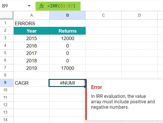
#NUM error
For instance, consider the above IRR example. If you do not change the initial value to a negative value, you get the #NUM error.

#NAME error
For any invalid arguments, like entering alphabets or other wrong entries, you get the #VALUE error.

Important Things to Note
- The three primary input values of importance when using different functions to calculate the CAGR include the investment beginning value, the ending value, and the time period.
- The average annual growth rate in arithmetic mean that can be calculated using the AVERAGE function, while the CAGR is a smoothed-out growth rate that is steady.
- Among the different methods specified above to calculate the CAGR formula in Google Sheets, the IRR method is the fastest and most straightforward.
- A company’s revenues or share price with a 10% CAGR means that it has grown in value at 0% average annually over the period specified.
Frequently Asked Questions (FAQs)
CAGR (Compound Annual Growth Rate) is the compounding effect over a specific period and is a fixed number. It is used to smooth out year-to-year fluctuations and provides a single growth rate over the entire period. The annual average growth rate is a simple average of the growth rates which can vary yearly without considering compounding effects.
The CAGR helps in the following ways.
• It helps you set clear goals in your investments.
• Helps you set proper money goals.
• It helps businessmen compare their revenues with their competitors helping make informed decisions about future growth.
Some of the common mistakes which can be avoided when calculating the CAGR
formula in Google Sheets include: Incorrect formula usage: Since we use different formulas such as URR, RATE etc, it is important to understand the syntax and use the correct arguments.
Misinterpreting results: You should never take the CAGR result at face value. Analyze other conditions such as the consistency of growth, noted periods of decline, appropriate time frame, etc. before arriving at a decision.
As mentioned above, there may be various factors which may contribute to CAGR not being analyzed accurately. These include assumption of a fixed growth rate over the years, not capturing the volatilities during this period, etc. Hence, all these factors should be considered before making any decision.
Download Template
📥Download the ready-to-use Excel template to practice this tutorial yourself.
CAGR Formula in Google SheetsRecommended Articles
This has been a guide to CAGR Formula in Google Sheets. Here we explain the how to use CAGR Formula in Google Sheets with its examples & points to remember. You can learn more from the following articles –

Leave a Reply