
What Is Carriage Return In Excel?
The Carriage Return in Excel helps users add a line break of the text inside a single cell and avoids jumping to the next line. The shortcut key used is “Alt+Enter”.
The Excel Carriage Return can also be inserted using the CHAR and TRIM functions to display the required cell value, sentence, or paragraph, in an orderly and organized manner.
Use this Carriage Return In Excel Template to follow along with the examples in this article.
Download Excel TemplateFor example, the image below shows the String, and we will insert Carriage Return using the keyboard shortcut keys ALT + Enter.

Copy the text from cell A2, and paste it to cell B2.
Now, select cell B2, and place the cursor before “Banana”, as shown below.

Press the keyboard shortcut key “ALT + Enter”.

The result is shown above. The text “Apple” is in the first line, and “Banana” moved to the second line, within the same cell, because the line break was placed before the “Banana” string.
Key Takeaways
- The Carriage Return in Excel is a line break feature that breaks the text in a group of strings within a cell, and moves it to the next line inside the same cell.
- We can insert and remove the Carriage Return using other Excel formulas, like the CHAR, TRIM, and SUBSTITUTE functions.
- The shortcut to insert the Carriage Return is Alt+Enter, and to remove is Ctrl+J in the “Find & Replace” dialog box.
- We can use the shortcut keys “ALT + Enter” twice to insert a double space.
Explanation And Uses Of Carriage Return In Excel
Explanation of Carriage Return
- In Excel, when we press “Enter”, the cursor jumps to the next line. So, to break the data and move it to the next line, or to add a new line for text within the same cell, we use the shortcut key “ALT + Enter” to insert the Carriage Return and start the text on the next line.
Uses of Carriage Return
- It helps us display text or a paragraph in an order.
- It helps us add extra spaces between lines of text.
How To Insert Carriage Return In Excel?
We can insert Carriage Return as follows,
- In the selected cell, take the cursor where we want a line break in excel, and press the excel shortcut keys “Alt+Enter”.
- We use the Excel functions such as CHAR and TRIM in excel in a formula to add line breaks.
The image below shows the name and addresses of the people, and we will insert Carriage Return using the CHAR function in Excel.
In the table, the data is,
- Column A: Contains First Name
- Column B: Contains Last Name
- Here, column C: Contains Street
- Column D: Contains City
- Column E: Contains State
- Here, column F: Contains Postal Code
- Column G: Contains Full Address

The steps to insert the Carriage Return inside excel cell using Char() are as follows:
- Select cell G2, and enter the formula,
=A2&“ ”&B2&CHAR(10)&“ ”&C2&CHAR(10)&“ ”&D2&“ ”&E2&“ ”&F2.

- Press the “Enter” key. The result is shown below,
“Ron Weasly
34, Davidson Ave.
Chicago IL 60007”.
- Drag the formula from cell G2 to G5 using the fill handle. The output is shown below.


Examples
We will see some advanced scenarios using the Carriage Return in Excel examples.
Example #1 – Using the CHAR Formula
The image below shows two numerical values in two different cells, and we will insert Carriage Return on the Numerical values using the Char() formula.
In the table, the data is,
- Column A: Contains Value 1
- Here, column B: Contains Value 2
- Column C: Contains Output

The steps to insert the Carriage Return and Char are as follows:
- Step 1: Select cell C2, and enter the formula =A2&CHAR(10)&B2.

- Step 2: Press the “Enter” key. The result is shown below.
“10
20”

Example #2
The image below shows the String, and we will insert Carriage Return using the keyboard shortcut keys ALT + Enter in Excel.
In the table, the data is,
- Column A: Contains String
- Column B: Contains Output

- First, copy the string from cell A2 and paste it to cell B2.
- Next, select cell B2, and place the cursor before the text “wait”.

- Press the keyboard shortcut key “ALT + Enter”.

The result is shown above. “Time and Tide” is in the first line, and “wait for none” is in the second line because the line break was placed before the string “wait”.
How To Remove Carriage Return In Excel?
We can remove the Carriage Return as follows:
- Select a data cell, press “Ctrl+H” to open the “Find & Replace” dialog box,
- Press the shortcut keys “Ctrl+J” in the “Find what” field.
- Type the line break characters comma(,), semi-colon(;), etc., in the “Replace with” field.
- Click the “Replace” button.

As seen in the above image, in the “Find what” field, a small blinking line appears, indicating that the Carriage Return shortcut is used.
It will join all selected cells into one cell, therefore, removing the line breaks.
For Example, the image below shows the String, and we will remove Carriage Return using the keyboard shortcut keys “CTRL + H” and “CTRL +J” in Excel.
In the table, the data is,
- Column A: Contains Initial Text
- Here, column B: Contains Text
- Column B: Contains Output

The steps to remove the Carriage Return in Excel are as follows:
- Step 1: First, we will insert the Carriage Return.
Copy text from cell A2, paste it to cell B2, place the cursor before “Potter”, and press the keyboard shortcut key “ALT + Enter”.
The result shown below shows “James” in the first line and “Potter” in the second line because the line break was placed before the “Potter” string.

- Step 2: Now, we will remove the Carriage Return.
- Copy cell B2, and paste it to cell C2.
- Press the keyboard shortcut keys “CTRL + H” to open the “Find and Replace” dialog box.
- In the “Find and Replace” box,
- Press the keyboard shortcut “CTRL + J” keys in the “Find What” box, and the small cursor appears.
- Click the “Replace All” button, as shown below.

Therefore, the Carriage Return is removed, as shown in the below image.

Important Things To Note
- The Carriage Return inserts the line break within a single cell.
- The formula for entering the Carriage Return is the CHAR(10) allows us to add the carriage return within a cell using the formula.
- We can also use Excel’s TRIM() or SUBSTITUTE excel function to remove carriage returns from a cell.
Frequently Asked Questions (FAQs)
The formula for the Carriage Return is the CHAR(10).
Let us explain using the example of the image below shows employees’ details, and we will insert Carriage Return using the CHAR function in Excel.
In the table, the data is,
• Column A: Contains Name of Employees
• Column B: Contains Year
• Here, column C: Contains City
• Column D: Contains Output
The steps to insert the Carriage Return and Char() are as follows:
• 1: Select cell D2, and enter the formula =A2&“ ”& CHAR(10)&“ ”&B2& CHAR(10)&“ ”&C2.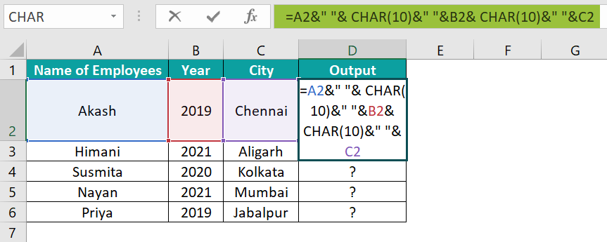
• 2: Press the “Enter” key. The result is shown below.
“Akash
2019
Chennai”.
• 3: Drag the formula from cell D2 to D6 using the fill handle. The output is shown below.
The Shortcut Keys for inserting Carriage Return in Excel are ALT + Enter.
The Shortcut Keys for removing Carriage Return in Excel are,
• CTRL + H keys to open the “Find and Replace” window.
• CTRL + J keys to remove.
The image below shows the price of fruits, and we will fix Carriage Return using the CHAR function and the TRIM function in Excel.
In the table, the data is,
• Column A: Contains Fruits
• Column B: Contains Price
• Here, column C: Contains Insert Output
• Column D: Contains Remove Output
The steps to evaluate the result using the Carriage Return Excel are as follows:
• 1: Select cell C2, and enter the formula =A2&“ ”& CHAR(10)&“ ”&B2.
• 2: Press “Enter”, and drag the formula from cell C2 to C6 using the fill handle, as shown below.
• 3: Select cell D2, and enter the formula =TRIM(C2).
• 4: Press “Enter”, and drag the formula from cell D2 to D6 using the fill handle. The output is shown below.
Use this Carriage Return In Excel Template to follow along with the examples in this article.
Download Excel Template