CORREL Function

What Is CORREL Function In Excel?

The CORREL function in Excel determines the correlation coefficient of two datasets or variables, where the coefficient value lies between -1 and 1. The function helps to evaluate the relationship between two variables, such as height and weight, price and sales, a specific stock and market index, etc.

The Excel CORREL function is an inbuilt Statistical function, so we can insert the formula from the “Function Library” or enter it directly in the worksheet.

For example, using the CORREL function in Excel, we will find the correlation between the two variables, i.e., the height and weight values given in the following table.

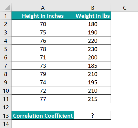
Select cell B13, enter the formula =CORREL(A2:A11,B2:B11), and press “Enter”.

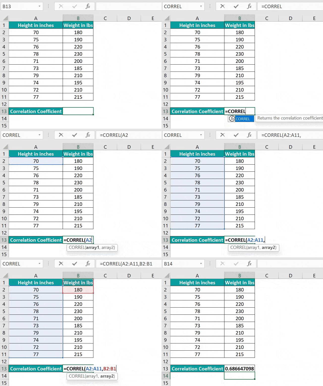
The result is 0.686647098, as shown below. A positive correlation coefficient implies that the two given datasets are proportionate, i.e., the more the height, the higher the weight.

What Is CORREL Function In Excel?

The CORREL function computes the correlation coefficient of the two specified arrays, two cell ranges representing different variables.
The correlation coefficient can be a value from -1 to 1.
- If the output is greater than 0, the correlation between the two given datasets is Positive.
- If the coefficient value is less than 0, the correlation between the two given datasets is Negative.
If the coefficient value is exactly 1 or -1, it indicates that the correlation between the two given arrays is perfectly positive or negative.

CORREL() Excel Formula

The syntax of the Excel CORREL Formula is,

The arguments of the Excel CORREL formula are,

array1: The first dataset or cell range of the first variable. It is a mandatory argument.
array2: The second dataset or cell range of the second variable to find the correlation with the first variable. It is a mandatory argument.

Excel VBA – All in One Courses Bundle (35+ Hours of Video Tutorials)

If you want to learn Excel and VBA professionally, then Excel VBA All in One Courses Bundle (35+ hours) is the perfect solution. Whether you’re a beginner or an experienced user, this bundle covers it all – from Basic Excel to Advanced Excel, Macros, Power Query, and VBA.

Start Learning Now

How To Use CORREL Excel Function?

We can use the CORREL Excel Function in 2 ways, namely,

Access from the Excel ribbon.
Enter in the worksheet manually.

Method #1 – Access from the Excel ribbon

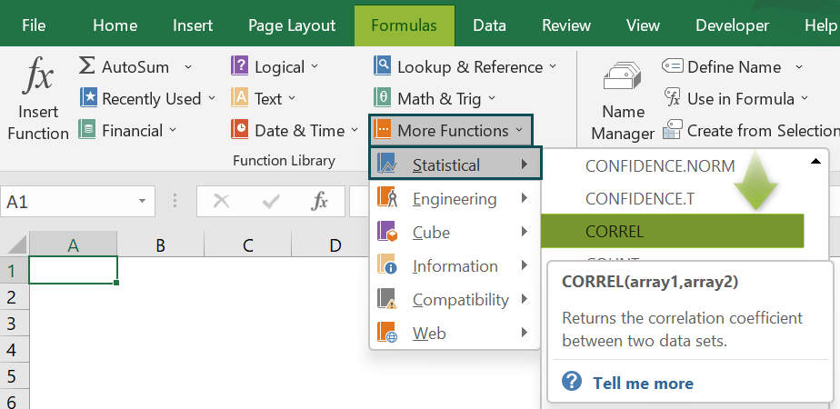
Choose an empty cell for the output → select the “Formulas” tab → go to the “Functions Library” group → click the “More Functions” option drop-down → click the “Statistical” option right-arrow → select the “CORREL” function, as shown below.

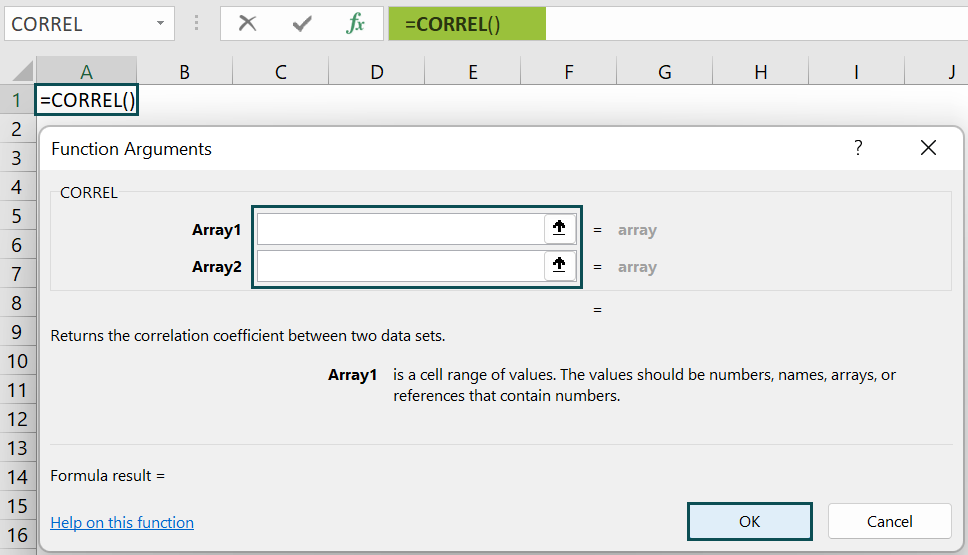
CORREL Function - access from the excel ribbon

The “Function Arguments” window opens. Enter the arguments in the “Array1” and the “Array2” fields → click “OK”, as shown below.

Method #2 – Enter in the worksheet manually

The steps to enter the CORREL excel function are as follows:

Select an empty cell for the output.
Type =CORREL( in the selected cell. [Alternatively, type =C or =COR and double-click the CORREL function from the Excel suggestions.]
Enter the arguments as cell values or cell references in excel.
Close the brackets and press Enter to get the result.

Let us understand this function using a basic example.

We will find the correlation between the two variables using the CORREL function.

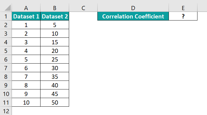
The table below contains two datasets.

How to Use CORREL Excel Function - Basic Example

The steps to find the correlation using CORREL excel function is,

Select cell E1, and enter the formula =CORREL(A2:A11, i.e., A2:A11 is the first variable’s cell range.
In continuation with the formula, select B2:B11, i.e., the second variable’s cell range, and close the bracket. The complete formula is =CORREL(A2:A11,B2:B11).
Press “Enter”. We will get the result as 1, as shown below

[Alternatively, we can apply the CORREL function using the option in the Formulas tab. First, select cell E1 and go to Formulas → More Functions → Statistical → CORREL to open the Function Arguments window.

We must enter the CORREL excel function argument values in the Function Arguments window.

And once we click OK in the Function Arguments window, the CORREL() will get executed in the target cell.
[Output Observation: The CORREL function output in the above example is 1, interpreting that the correlation between the two datasets is perfect positive. In other words, the two perfectly correlated datasets vary linearly, and all the data points lie in a straight line.]

Examples

We will understand some advanced scenarios using the CORREL function in Excel examples.

Example #1

The mathematical representation of the CORREL function is:

mathematical representation of CORREL function

The x_mean and y_mean are the means of X and Y datasets (array1 and array2).

This example shows how the above mathematical expression works and results in the same correlation coefficient as the CORREL excel function.

The first table contains age-height values. While the age values form the x dataset (array1), the weight values form the y dataset (array2).

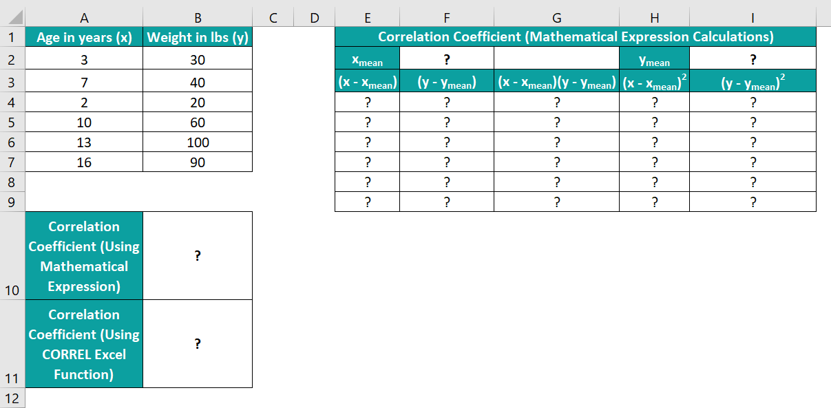
We will calculate the correlation coefficient for the age-weight data using the CORREL() mathematical expression in cell B11 and the CORREL function formula in cell B12 as follows:

Step 1: Select cell F2, enter the formula =SUM(A2:A7)/6 to determine the average age, and press Enter. We get the result as 8.5, as shown below.

Step 2: Next, select cell I2, enter the formula =SUM(B2:B7)/6 to determine the average weight, and press Enter. We get the result as 56.67, as shown below.

Step 3: Select cell E4, enter the formula =A2-$F$2, and press Enter. We get the result as -5.5, as shown below.

Step 4: Drag the formula from cell E4 to E9 using the fill handle.

Step 5: Next, select cell F4, enter the formula =B2-$I$2, and press Enter. We get the result as -26.67, as shown below.

Step 6: Then, drag the formula from cell F4 to F9 using the fill handle.

Step 7: Select cell G4, enter the formula =E4*F4, and press Enter. We get the result as 146.67, as shown below.

Step 8: Drag the formula from cell G4 to G9 using the fill handle.

Step 9: Again, select cell H4, enter the formula =E4*E4, and press Enter. We get the result as 30.25, as shown below.

Step 10: Here, drag the formula from cell H4 to H9 using the fill handle.

Step 11: Select cell I4, enter the formula =F4*F4, and press Enter. We get the result as 711.11, as shown below.

Step 12: Drag the formula from cell I4 to I9 using the fill handle.

Step 13: Finally, we will use the CORREL() mathematical expression as we have calculated all the required values.

Select cell B11, enter the formula =SUM(G4:G9)/SQRT(SUM(H4:H9)*SUM(I4:I9)), and press Enter.

We will get the following output.

14: Now, we will find the correlation using the CORREL formula.

Select cell B12, enter the formula =CORREL(A2:A7,B2:B7), and press Enter.

Thus, the two formulas in cells B11 and B12 give the same correlation coefficient, 0.95048419.

Example #2

In this example, we will see how to determine the correlation coefficient using the CORREL function and plot the data points to check the correlation trend.

The below table shows the values of two datasets, X and Y.

The steps to find the correlation between the two variables using the CORREL function in excel, and to graphically represent the trend using the Scatter plot, are as follows:

Step 1: Select cell D2, enter the formula =CORREL(A2:A11,B2:B11), and press Enter. The result is 0.893437198, as shown below.

Step 2: To create a chart, choose the cell range A1:B11 → select the “Insert” tab → go to the “Charts” group → click the “Insert Scatter (X, Y) or Bubble Chart” option drop-down → select the “Scatter” chart type from the “Scatter” group, as shown below.

Step 3: Click the chart to enable the Chart Elements (‘+’ icon) and select the options shown below.

Step 4: Update the chart and axes titles using the respective elements in the chart area, as required.

And thus, the final Scatter plot is shown below. The trendline shows a positive correlation between the given X and Y datasets. It implies that as the X array values increase, the Y array values increase.

Step 5: Let us see the Scatter plot trendline for a negative correlation coefficient. And for that, assume the new X and Y datasets and the corresponding CORREL function output in cell D2 are as follows:

Now, create the Scatter plot as explained in steps 2, 3, and 4 for the above datasets. The calculated correlation coefficient between the new datasets is negative, shown below in the trendline in the graph.

Step 6: Let us see the Scatter plot trendline for zero correlation coefficient. And for that, assume the new X and Y datasets and the corresponding CORREL function output in cell D2 are as follows:

Now, create the Scatter plot as explained in steps 2, 3, and 4 for the above datasets.

The calculated correlation coefficient between the new datasets is 0. And the trendline in the Scatter plot confirms the no correlation between the two datasets.

Example #3

This example shows how the CORREL function behaves when the supplied arrays are of different sizes, negative or empty.

The following table contains the ten weeks of stock N and S & P weekly change data.

We will find the correlation coefficient between the two given datasets with some scenarios as follows:

Scenario 1: #N/A error if the array1 and array2 sizes are unequal.

Select cell E2, enter the formula =CORREL(B2:B9,C2:C11), and press “Enter”. The result is the #N/A error. The reason is that the array1 and array2 sizes are unequal.

When we enter the right size array ranges, then the function executes correctly. We get the coefficient value as 0.236194374, as shown below.

Scenario 2: Some cells in the above-given datasets are empty, but the two supplied array ranges are correct. The function ignores such cells to return the correlation coefficient value for the provided data points.

For example, the two datasets with empty cells are:

Select cell E2, enter the formula =CORREL(B2:B11,C2:C11), and press Enter. The output will be

–0.923506323, as shown below. The correlation between them is negative.

Scenario 3: If one of the datasets is empty, as depicted in the image below.

Select cell E2, enter the formula =CORREL(B2:B11,C2:C11), and press Enter. The result is #DIV/0! Error, as shown below.

Thus, when we supply two datasets of the same size, with all the data points accurate, to the CORREL(), it will return the correct correlation coefficient value.

Important Things To Note

The CORREL function in excel ignores cells containing text or logical values and empty cells. But it considers cells containing zero value.
If we supply two datasets of different array sizes to the CORREL(), it returns the #N/A error.
If any datasets are empty or the standard deviation of the given data points is 0, the CORREL function throws the #DIV/0! error.

Frequently Asked Questions (FAQs)

1. Where is the CORREL function in Excel?

The CORREL function in Excel is in the Formulas tab. Go to Formulas → More Functions → Statistical → CORREL to apply the function in the target cell.

2. Why is the CORREL function not working in Excel?

The CORREL function may not work for the following reasons:
• The provided arrays have different sizes.
• If the provided arrays are empty.
• The standard deviation of the data points in the given datasets is 0.

3. How do we apply the CORREL function in Excel VBA?

We can apply the CORREL function in Excel VBA using the method:

Application.WorksheetFunction.Correl(array1,array2)

For example, the table below shows the number of hours studied and marks secured out of 100.

The steps to apply the method for the CORREL() in Excel VBA are as follows:

• 1: In the worksheet with the above table open, press the keys Alt + F11 to access the VBA Editor.

• 2: Pick the required VBAProject and select Insert → Module to open a new module, Module1.

• 3: In the newly opened module window, enter the VBA code, shown in the image below.

Sub CORREL_fn()
Range(“B12”) = Application.WorksheetFunction.Correl(Range(“A2:A10”), Range(“B2:B10”))
End Sub

• 4: Click the Run Sub/UserForm icon to run the VBA code.

• 5: Finally, open the active worksheet to view the result in the target cell.

The method in the above VBA code accepts the two given cell ranges as array1 and array2 and determines their correlation coefficient as 0.876071679.

Download Template

This article must help understand the CORREL function, with its formula and examples. We can download the template here to use it instantly.

CORREL Function Download

CORREL Function