
What is CRITBINOM in Google Sheets?
CRITBINOM in Google Sheets is a statistical function used to calculate the critical value for a binomial distribution. It is used to find the smallest number of successes needed for the cumulative binomial probability to be greater than or equal to a specified criterion. In other words, it finds the number of successes needed for a given probability. This makes it very useful in applications in quality control, where one can find the minimum number of acceptable products in a batch, or in research to find the threshold at which a certain result becomes statistically significant.
The function can be called the inverse of the cumulative binomial distribution and requires three arguments: the number of trials, the probability of success for each trial, and the criterion value, which is a probability threshold. For example, if you have 100 trials with a 50% probability of success and a criterion of 10%, CRITBINOM will return the smallest number of successes, which is 44, for which the cumulative probability is at least 10%.
For this, we write the formula: =CRITBINOM(B1,B2,B3). It helps users analyze the likelihood of specific outcomes and make informed decisions based on probabilistic thresholds.

Use this CRITBINOM in Google Sheets Template to follow along with the examples in this article.
Download Excel TemplateKey Takeaways
- CRITBINOM in Google Sheets returns the smallest number of successes for which the cumulative binomial distribution is greater than or equal to a specified probability threshold.
- The syntax of the function is as follows: =CRITBINOM(trials, probability_s, alpha)
trials – The total number of independent trials.
probability_s – The probability of success in each trial.
alpha – The target cumulative probability.
- CRITBINOM is useful for finding the cutoff point needed to meet a desired confidence level in risk assessment, quality control, or forecasting.
- It requires all arguments to be numeric, and the probability values must fall between 0 and 1 for valid results.
Syntax
The CRITBINOM in Google Sheets formula is as follows:
=CRITBINOM(num_trials, prob_success, target_prob)
- num_trials – The number of independent trials.
- prob_success – The probability of success in any given trial.
- target_prob – The desired threshold probability.
How To Use CRITBINOM Function in Google Sheets?
CRITBINOM in Google Sheets is used to find the minimum number of successful outcomes required in a fixed number of independent trials to achieve a specified cumulative probability. It’s useful in probability analysis, risk assessment, and scientific testing where one must determine how many successes are needed to reach a given confidence level.
CRITBINOM can be entered manually or by using the Google Sheets menu.
Entering CRITBINOM Manually
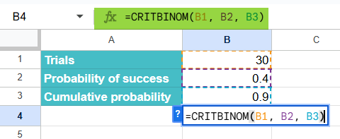
Let us consider a scientist who conducts 20 trials of an experiment where each trial has a 40% chance of success. The scientist wants to determine the minimum number of successful outcomes needed so that there is at least a 90% probability of achieving that number or fewer successes.
Step 1: Enter the values into a Google Sheet, as shown below.

Step 2: Click on an empty cell and type the following formula:
=CRITBINOM(B1, B2, B3)
Step 3: Press Enter. The result will be 15, meaning that at least 15 successful outcomes are required in 20 trials to reach a cumulative probability of 90%.

This tells the scientist that there is a 90% chance of getting 15 or fewer successes, helping to set realistic expectations for the experiment’s outcomes.
Using CRITBINOM From the Google Sheets Menu
- Select the cell where you want the result to appear.
- Go to Insert → Function → Statistical.
- Scroll down and choose CRITBINOM.
- Enter the values for number_s, probability_s, and cumulative (in this order).
- Press Enter to get the minimum number of successes required.
Examples
Let us look at some practical examples of how the CRITBINOM function can be used in Google Sheets.
Example #1 – Calculate the Minimum Number of Successes Required in a Certain Number of Scientific Trials
A research team is running 20 genetic experiments, each with a 40% chance of success. They want to find the minimum number of successful outcomes needed so that there is a 90% probability of achieving that number or fewer successes.
Step 1: Enter the values in the Google Sheet, as shown below.

Step 2: In a blank cell, enter the following formula:
=CRITBINOM(B1, B2, B3)

Step 3: Press Enter. The result will be 11, meaning that in 20 trials, the researchers can expect at least 11 successful experiments with a 90% probability.

The CRITBINOM result helps the research team set a performance which helps them plan resources and interpret their results with greater statistical confidence.
Example #2 – Determine the probability of achieving a certain number of successes for a football team in a tournament
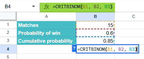
A football coach wants to analyze the team’s chances in an upcoming 15-match tournament. Analysis of the past performance shows that the team has a 60% chance of winning each match. The coach wants to find the minimum number of matches the team needs to win to have at least an 85% probability of achieving that or fewer wins.
Step 1: Enter the tournament data in a Google Sheet.

Step 2: Click on a blank cell and type the formula:
=CRITBINOM(B1, B2, B3)
Step 3: Press Enter. The result will be 11, meaning that with a 60% win rate, the team can expect to win up to 11 matches with an 85% probability.

The coach can use this insight to set realistic expectations. Winning more than that would signal an above-average performance, indicating the training strategy is working effectively.
Example #3 – Calculate the risk of a certain outcome in an insurance
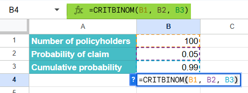
An insurance analyst is evaluating the risk associated with 100 policyholders, each having a 5% probability of filing a claim each year. The company wants to determine how many claims they might expect with 99% certainty — to plan their reserve funds accordingly.
Step 1: Enter the insurance data in a sheet as follows.

Step 2: Enter the following formula in an empty cell.
=CRITBINOM(B1, B2, B3)
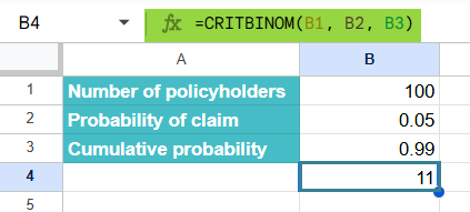
Step 3: Press Enter. The result will be 11. This means that the insurer can expect up to 11 claims per year with a 99% certainty.
Step 4: To visually analyze this, one can use conditional formatting.
- Highlight the cell containing the result (e.g., B4).
- Go to Format → Conditional formatting.
- Under Format rules, choose “Custom formula is.”
- Enter the formula: f. (8 is the threshold risk we chose)
Choose a color fill to highlight values above the threshold. Click Done.

The analysis shows that with 99% confidence; the insurer should expect up to 11 claims annually.
Important Things to Note
- The second argument, the probability of success represents the probability of success in one try. It is a value between 0 and 1, with 0 representing impossible success and 1 representing definite success.
- We use CRITBINOM in financial decision-making to assess the probability of a specific number of profitable investments or events occurring in a financial portfolio.
- CRITBINOM is very useful for decision-making and risk assessment and is used for the same in project management and manufacturing.
Frequently Asked Questions (FAQs)
Though the function is not as popular as functions like VLOOKUP, CRITBINOM has its own place in statistical analyses. It can be used in hypothesis testing and decision making. By using CRITBINOM, users can accurately determine the critical value for a binomial distribution. Thus, it is a valuable tool for data analysis.
1. It is used in risk analysis to estimate the minimum number of successful outcomes needed to achieve a target probability in financial models.
2. Its role in quality control is very crucial as it can find the acceptable defect levels in manufacturing before a product batch is approved.
3. Researchers use it for scientific experiments to decide how many successful trials are required to validate experimental results.
4. In sports analysis, it helps predict how many wins a team requires to reach a certain success probability in tournaments.
BINOMDIST calculates the probability of getting a specific number of successes in a particular number of trials. It’s useful when you want to know how likely an event is to occur a certain number of times.
Syntax: =BINOMDIST(number_s, trials, probability_s, cumulative)
The cumulative argument determines whether you want the exact probability (FALSE) or cumulative probability (TRUE).
CRITBINOM is the opposite; it returns the minimum number of successes needed to reach a specified cumulative probability. It’s helpful when you want to know how many successes are required to meet a certain confidence level.
=CRITBINOM(trials, probability_s, alpha)
We have the following errors:
1. VALUE! error: This error occurs if any of the given arguments are not numbers. If the test argument is a decimal, it is truncated.
2. The NUM! error: We get this error when the test argument is less than 0. Also, if the given probability is less than zero or greater than one; or the given alpha argument is less than zero or greater than one.
CRITBINOM can be combined with functions like IF or ARRAYFORMULA to automate probability-based thresholds. It is therefore useful for simulations, forecasting, and decision modeling.
Use this CRITBINOM in Google Sheets Template to follow along with the examples in this article.
Download Excel Template