EDATE Excel Function

What is EDATE Function in Excel?

The EDATE function in Excel is an inbuilt Date & Time function. It returns the serial number representing the date, the indicated number of months before or after a given date. Users can use the EDATE function to calculate values such as maturity dates falling on the same day as the issue date.

For example, consider the below table. It shows a list of dates in column A, entered using the DATE(). And column B contains the number of months to get the required date before or after the given date.

Suppose we must determine the dates according to the comments in column C and display the output in the target cell range D2:D6. Then using the data in columns A and B, we can perform the EDATE Excel function calculation in each target cell to get the required dates.

According to the EDATE function logic, the function returns the date based on the specified number of months before or after the initial date. In addition, as mentioned in the definition, the EDATE() returns the serial number of the determined date. Therefore, we can set the data format of the target cells as Short Date in the Home tab, as highlighted in the above image, to view the EDATE() output in the proper date format in excel.

What is EDATE Function in Excel?

EDATE Excel Function is an inbuilt Date & Time function.
The formula of EDATE excel is =EDATE(start_date,months)
The EDATE() accepts two mandatory arguments as input, start_date and months. While the start_date is a date value, months can be a positive or negative numeric value.
Users can apply the EDATE() in calculations, such as determining the maturity dates falling on the same day in a month as the initial date.
We can use the EDATE() more effectively by applying it along with other Excel functions such as IF, COUNTIFS, and YEARFRAC.

EDATE() Excel Formula

The EDATE Excel formula is:

where,

start_date: The date representing the initial or start date.
months: The number of months before or after the start date. The EDATE Excel function returns a future date for the positive value of the argument months. And the function output will be a past date for a negative value.

Both the EDATE Excel function arguments are mandatory.

We must consider the following critical points while calculating the EDATE Excel function calculation.

It is best to enter the start date using the DATE Excel function, as it ensures the date is not a text value and the EDATE Excel function works properly.
If the start_date is an invalid Excel date or the arguments provided to the EDATE() are non-numeric, the function will throw the #VALUE! error.
If the supplied months argument is not an integer, it gets truncated during EDATE function execution.
If the applied EDATE logic results in an invalid date, the function output will be the #NUM! error.

Excel VBA – All in One Courses Bundle (35+ Hours of Video Tutorials)

If you want to learn Excel and VBA professionally, then Excel VBA All in One Courses Bundle (35+ hours) is the perfect solution. Whether you’re a beginner or an experienced user, this bundle covers it all – from Basic Excel to Advanced Excel, Macros, Power Query, and VBA.

Start Learning Now

How to Use EDATE Excel Function?

Adhere to the below steps while using the EDATE Excel function.

First, confirm the source data contains the start date and months we provide, as the EDATE Excel function arguments are in the required formats.
Then, select the target cell, enter the EDATE(), and press Enter.
Finally, select the target cell containing the serial number of the resulting date and set the data format as Date to view the EDATE() output as a date value.

Let us see the above steps using an EDATE Excel function example.

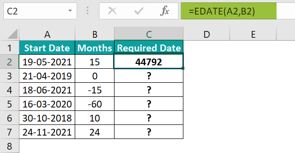
Consider the following table containing a list of start dates and the number of months before or after the start dates we require the date.

And suppose we have to display the required dates in the target cell range C2:C7. Then we can apply the EDATE() in the target cells, and the steps are as follows:

Select the target cell C2, enter the EDATE() provided in the Formula Bar in the below image, and press Enter.

We can also execute the EDATE() by selecting the target cell C2 and clicking Formulas → Date & Time → EDATE to open the Function Arguments window.

Next, enter the two argument values in the Function Arguments window.

And once we click OK in the Function Arguments window, we will view EDATE() output.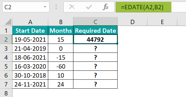

The EDATE Excel function returns the date’s serial number 15 months after the given start date, 44792. So, we need to set the target cell data format as Date.
Select cell C2, click the Number Format drop-down button in the Home tab and select the Short Date format.
Drag the fill handle downwards to copy the formula in cell range C3:C7.

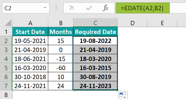
We can see that when the argument months is 0, the EDATE() returns the start date as the output, as there are no months to add or subtract from the given start date.

Examples

Let us see some example scenarios where we can apply the EDATE() and make the best use of it.

Example #1

The below table contains a list of items, their manufacture dates, and shelf life details.

And suppose we have to determine their respective expiry dates and display the results in the target cell range D2:D5. Then applying the EDATE Excel function in the target cells, we can get the required dates.

Step 1: Select the target cell range D2:D5 and set the Number Format option in the Home tab as Short Date. It will ensure the EDATE function output is in the date format rather than serial numbers representing the resulting date values.

Step 2: Select the target cell D2, enter the following EDATE(), and press Enter.

=EDATE(B2,C2)

Step 3: Drag the fill handle downwards to copy the formula in cell range D3:D5.

In the above example, the date of manufacture and shelf life are the start_date and months arguments for the EDATE(). And based on these two inputs, the function returns the required date in the target cells.

Example #2

Consider the first table in the image below. It shows a list of activities and the target dates to complete them.

Please Note: The target dates data format in column B is Date.

And, the column D month data has a custom date format, mmm-yy.

Here is how we can set the above custom format.

Select the required cell, click the Number Format drop-down list in the Home tab and choose the More Number Formats option to open the Format Cells window.

In the Format Cells window, choose the Custom option in the Number tab and pick the required format, as highlighted in the image below. And finally, click OK to apply the format.

EDATE Excel Function - Example 2-Format Cells

Suppose the requirement is to determine the number of activities we must complete each month based on the first table data and display the results in column E of the second table. In such a scenario, use the EDATE in the COUNTIFS excel function to populate the required date values in column E.

Step 1: Select the target cell E2, enter the below formula, and press Enter.

=COUNTIFS(($B$2:$B$19),”>=”&D2,($B$2:$B$19),”<“&EDATE(D2,1))

Step 2: Drag the fill handle downwards to copy the formula in the cell range E3:E13.

Let us consider the target cell E13 to see how the formula works. First, the COUNTIFS() checks for cells in the cell range B2:B19 where the dates are greater than or equal to 1-12-2020 (Dec-20). So, in this case, the first condition holds in cells B17:B19. Then the EDATE() returns the date one month after 1-12-2020 (Dec-20), that is, 1-1-2021 (Jan-21). The COUNTIFS() now checks the cell range B2:B19 for cells where the first condition holds and the dates are less than 1-1-2021. In this case, the second condition holds in all three cells B17:B19, and thus the function returns the value 3.

Please note that in the above example, the first condition in the COUNTIFS() holds for some cells in the given cell range B2:B19. And that is why the function checks the second condition. Otherwise, the function would return 0 as the output.

Example #3

The below table shows an employee list and their details.

Suppose we need to find the employees who will retire in a year, based on their date of birth, and display the results in column D. Then, we can achieve the required output using the EDATE and TODAY() in the YEARFRAC(), within the IF excel function.

Step 1: Select the target cell D2, enter the following IF() formula, and press Enter.

=IF(YEARFRAC(TODAY(),EDATE(C2,12*60))<=1,”Yes”,”No”)

Step 2: Drag the fill handle downwards to copy the formula in the cell range D3:D11.

Let us see how the formula works. Consider the formula in cell D11. The TODAY excel function returns the current date, say, 25-08-2022. Then the EDATE Excel functionreturn value is the date, 60 years after the given birth date (12-12-1962), 12-12-2022, as the retirement age in this example is 60 years. The YEARFRAC() determines the year fraction indicating the number of whole days between the given start and end dates. Here, the start and end dates are 25-08-2022 and 12-12-2022. So the YEARFRAC() output is 0.297, a value less than 1. Thus, the IF condition holds in cell D11, and the formula returns Yes.

So, we can use the EDATE() to determine the retirement year based on the input birth date.

Important Things to Note

The EDATE Excel function gives the date as a serial number, the indicated number of months before or after the given start date.
Ensure we enter the date value using the DATE(). It will help us avoid supplying the argument start_date as a text value to the EDATE Excel function.
For an invalid start_date or non-numeric arguments, the EDATE() returns the #VALUE! error.
If the argument months is not an integer, the EDATE() uses the truncated value as the argument.
If the EDATE() executes and determines an invalid date, the function throws the #NUM! error.

Frequently Asked Questions (FAQs)

1. Where is the EDATE function in Excel?

The EDATE function in Excel is in the Formulas tab. We can click Formulas → Date & Time → EDATE to access it.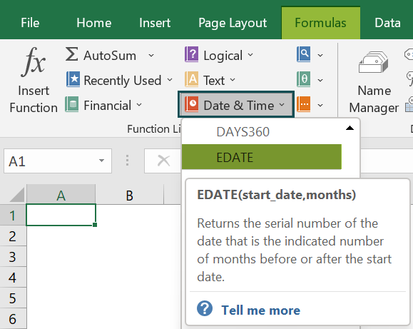

2. Why is my EDATE() not working?

If EDATE() is not working, it may be due to the following reasons.
• The start_date argument is not in the date format.
• The start_date argument provided to the EDATE() is invalid.
• The arguments supplied to the EDATE() as input are non-numeric.
• The EDATE() determined an invalid date.

3. Can you use EDATE() for years?

We can use EDATE() for years by multiplying the given number of years by 12 and using the resulting number of months as the second argument in the EDATE().

Let us see the steps with an example.

Assume we have to initiate a contract on 1-10-2022. And we have different contract terms in years, as depicted in the below image.

Suppose we have to calculate the contract termination dates based on the contract initiation dates and contract terms in the target cell range C2:C6. Then here is how we can apply the EDATE() to the target cells to get the required date values.

• Step 1: Select the target cell C2, enter the following EDATE(), and press Enter.
=EDATE(A2,12*B2)

• Step 2: Drag the fill handle downwards to copy the formulas in cell range C3:C6.

Let us consider the target cell C6 formula to understand how the EDATE() has worked for years. The start_date argument is a date value of 1-10-2022. While the unit of the contract term values is years, the second argument in the EDATE() is months. So, we can convert the contract term years into months to provide it as the second argument to the function. Since a year has 12 months, we multiply the given number of years, 12, by 12 months. The EDATE() then adds 144 months (12*12) to the given start_date to return the contract termination date as 1-10-2034, a date 12 years from 1-10-2022.

Download Template

This article must be helpful to understand the EDATE Excel Function, with its formula and examples. You can download the template here to use it instantly.

EDATE Excel Function Download

EDATE Excel Function