What Is Editing Drop-Down List In Excel?
An editing drop-down list in Excel is a powerful tool that allows users to select a value from a pre-defined list of options easily. It provides an efficient way to ensure data accuracy and consistency, particularly when multiple people work on the same spreadsheet. By creating a drop-down list, users can limit the input choices to only those valid for specific cells or columns, thus avoiding errors and reducing the need for manual data validation.
To ensure a smooth and user-friendly experience, it is crucial to have readily available drop-down values for input at each step. Let’s consider an example where our objective is to provide a selection of items. To achieve this, we must select a specific cell where we will insert the drop-down list.

For this purpose, let’s choose cell B2 as the location for our drop-down list. To proceed, navigate to the Data tab and locate the Data Tools section. Within this section, click on Data Validation in excel.
Next, click on Data Validation again in the Excel application, which will prompt a dialog box to appear. Select List under the Allow category within the dialog box’s Settings section.
Then, we must input the desired values in the designated source section to populate our drop-down options. Click OK.
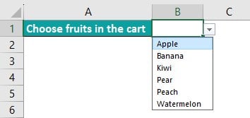
Now, we can see that our drop-down is created.

Table of contents
Key Takeaways
- The edit drop-down list in Excel helps users select a value from a pre-defined list of options.
- Editing drop-down lists in Excel can be customized to accommodate various requirements –allowing multiple selections, displaying dependent choices based on previous selections, or updating dynamically based on changes in the underlying data.
- This feature also streamlines data entry by offering predefined values instead of requiring users to type them out each time.
- In tables, the option to insert a new entry is available, which will automatically update the corresponding dropdown.
How To Edit Drop-Down List In Excel?
Editing the drop-down list in Excel is a fairly simple yet important task for professionals looking to enhance their data organization and analysis capabilities. Select the cell or cells containing the existing list to edit a drop-down list. Then, click the Data tab and choose Data Validation from the menu. In the Data Validation dialog box, go to the Settings tab and select List from the Allow dropdown menu. Here, we can manually update the entries in the Source field or use range references to refer to a specific column or set of cells containing our new list items. Ensure that we separate each item with a comma if manually editing them. Finally, click on OK to save and apply our modifications. This professional approach enables users to customize their drop-down lists without any hassle, improving efficiency and accuracy in data entry tasks within Excel spreadsheets.
Examples
Example #1 – Giving Drop Down Values Manually And Using Data Validation
To ensure a seamless user experience, we must have the drop-down values readily available for input during each step. Let’s consider an example where we aim to provide a selection of fruits. To achieve this, we must designate a specific cell where the drop-down will be inserted.
Step 1: Let’s choose cell B2 as the location for our drop-down list.

Step 2: Navigate to the Data tab and locate the Data Tools section. Within this section, click on Data Validation.

Step 3: Once again, click on Data Validation in the Excel application, which will prompt a dialog box to appear.
Step 4: Within the Settings section of the dialog box, select List under the Allow category.
Step 5: We must manually input the desired values for our drop-down options in the designated Source section.
Step 6: Upon clicking OK, our drop-down will be successfully created.

Step 7: The method above represents the simplest approach to creating and modifying a drop-down list in Excel. However, it is important to note that the entire process must be repeated if we need to add additional values to select fruits.
Example #2 – Giving Drop-Down Ranges And Using Data Validation
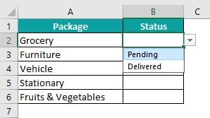
For instance, a set of products needs to be delivered. Consequently, I would like to include two options in the survey to track the delivery status: pending and delivered.
Step 1: While the method above serves its purpose, it is important to note that users can modify it by accessing the Data Validation tab and altering the values. We can hide the excel columns associated with the validation and dropdown to prevent such modifications, ensuring that other users cannot edit them.
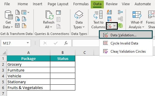
Step 2: To create the dropdown, we must copy or compile the values in a list or column. Once this is done, we can select the desired cell for validation, such as cell B2.
Step 3: Under the Data tab, within the Data Tools section, we should click on Data Validation. This action will prompt a wizard box to appear.
Step 4: We must select List under the Allow category within the settings. Subsequently, in the Source tab, we must choose the range of data that will populate the dropdown list.

Step 5: Click OK. We will be able to see a dropdown in cell B2. To extend this functionality till cell B6, we need to copy the validation accordingly. Ultimately, a dropdown list will be available in all the desired cells.
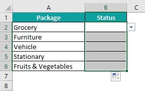
Step 6: Even if we hide the cell range serving as the dropdown source, it is important to note that users will still be unable to edit the validation. However, it is worth mentioning that this process shares the same drawback as the initial example. If we wish to include an additional option, such as Pending, we must repeat the entire process, including inserting a new alternative in the source and validation.
Example #3 – Creating A Data Table And Using Data Validation
In this method, we will demonstrate the creation of a data table and the utilization of data validation. To illustrate, let’s consider a scenario where different forms of clothes customers. I have conveniently inserted the relevant data in the column below.
Step 1: The first step is to create a table. Select the data and go to the Insert tab > Tables.
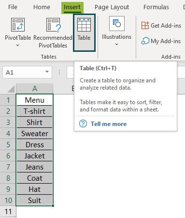
Step 2: Upon doing so, a window will appear, and by clicking OK, we will have successfully created our table in column A.

Step 3: Now, let’s assign a name to this table, such as Clothes. We can find an option to rename the table in the top left corner.

Step 4: We must select the cell where we want to insert the drop-down list.
Step 5: Under the Data tab, we will find the Data Validation option, which we must click on.
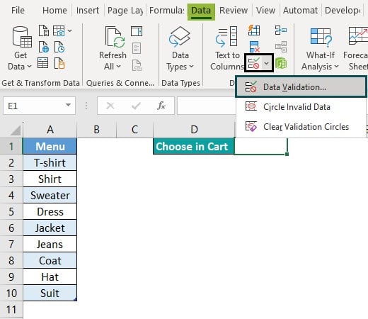
Step 6: Within the Allow tab, we should choose List.
Step 7: In the Source field, we must input the desired information as shown in the dialog box below.

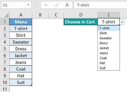
Step 8: Upon clicking OK, we will observe that a drop-down list has been inserted into the data.
Step 9: Suppose we have another menu to add, for instance, T-Shirt.
Step 10: We will notice that the new entry in the Menu tab is also shown within our drop-down list.
Explanation Of Edit Drop-Down List In Excel
The Edit Drop-Down List in Excel is a powerful tool that allows users to create a pre-defined set of options for data entry in a specific cell or range. This feature is particularly useful when working with large datasets or creating forms, as it ensures an accurate data input.
To use the Edit Drop-Down List, select the target cell(s) and then go to the Data Validation option under the Data tab. In the resulting dialog box, users can choose List as the validation criteria and specify the source of their dropdown options, either by manually entering them or referencing a range of cells. Moreover, advanced settings allow for error alerts if non-listed values are entered or restrict any changes to existing entries. The Edit Drop-Down List simplifies data entry tasks in Excel spreadsheets, making it an indispensable tool for professionals working with complex datasets.
Important Things To Note
- To ensure accurate data entry, it is necessary to either manually input drop-down values or establish predefined ranges.
- We have to create a fresh drop-down list for adding a new entry.
- To access and modify the drop-down list, click on the respective cell.

Frequently Asked Questions (FAQs)
In Excel, the maximum number of items allowed in a drop-down list depends on the Excel version used. In older versions of Excel, such as Excel 2003 and earlier, the limit is around 1,000 items per list. However, in newer versions like Excel 2007 and onwards, the limit has been increased significantly to accommodate up to approximately 32,767 items per list.
We can add items to a drop-down list in Excel by using data validation and VBA (Visual Basic for Applications).
For example, consider the below table. We will choose cell B2 as the location for our drop-down list. Select the Data tab > Data Tools > Data Validation.
Next, click on Data Validation again in the Excel application, which will prompt a dialog box to appear. Within the dialog box, select List under the Allow category in the Settings section.
Yes, we can remove the unwanted entries directly from the source data that populates the drop-down list.
First, go to the worksheet and select the cell containing the drop-down arrow. Next, click Data Validation under the Data tab.
Go to the Settings tab in the newly opened window. In the Source box, we will find all the values of our existing drop-down list. To remove a specific item, edit or delete its entry in this box.
Next, confirm the changes and click on OK. Now, when we access our drop-down menu again, we will notice that only the updated items remain selectable.
Download Template
This article must help understand Excel Edit Drop-Down List formulas and examples. We can download the template here to use it instantly.
Recommended Articles
This has been a guide to Edit Drop-Down List In Excel. Here we learn how to select values from pre-defined list of options with examples & downloadable template. You can learn more from the following articles –

Leave a Reply