Excel CEILING Function

What Is CEILING Function In Excel?

The CEILING function in Excel rounds up the numeric value from the dataset to its immediate or closest multiple as required or set in the formula. Users can use it to perform tasks, such as setting the rates after currency conversions during financial analysis.

The Excel CEILING function is an inbuilt Math & Trig function, so we can enter the formula directly in the worksheet or insert it from the “Function Library”. However, the CEILING.MATH() is replaced in Excel version 2013, and CEILING() is now available as a Compatibility function in Excel. For example, the below table shows a list of input values and the number rounding-up requirements.

Let us use the Excel CEILING function to get the rounded-up values. Select cell C2, enter the formula =CEILING(A2,7), and press the “Enter” key.

[Note: We entered the cell value instead of the cell reference. Therefore, we cannot drag the formula. So, insert the formulas shown in column D, in the column C cells, respectively.]

The output is shown above in column C, each as per the set multiple.

What is CEILING Function in Excel?

The Excel CEILING function rounds up the values, which may be any numeric value as fractions, integers, or negative numbers, to the nearest required multiple.
The CEILING() accepts two mandatory arguments as input, number, and significance.
For a negative number and significance, the CEILING() returns a number rounded down away from 0. And for a negative number and positive significance, the CEILING() rounds up the value towards 0.
We can use Excel conditional functions such as ISODD() and ISEVEN() along with the CEILING() function to apply conditional formatting and highlight the output.

CEILING() Excel Formula

The Excel CEILING formula syntax is:

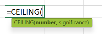
The Excel CEILING formula arguments are:

number: The numeric value we desire to round up. It is a mandatory argument.
significance: The multiple we require to round up the specified number. It is a mandatory argument.

[Special Note: The Excel CEILING function properties to understand before applying the function.]

Whether the supplied numeric value is positive or negative, the CEILING() will round it up to a value away from zero.
No rounding-up occurs if the number is an exact multiple of the specified significance value.
If both arguments are negative, the CEILING() rounds down the numeric value away from 0.
When the argument number is negative, and the argument significance is positive, the CEILING() rounds up the supplied number to a value closer to 0.
If the number argument is positive and the significance argument is negative, the CEILING() will return the #NUM! error.
The CEILING() will return the #VALUE! error, if we supply non-numeric arguments,
For the significance argument value of 0, the CEILING function output will be #DIV/0! error.

Excel VBA – All in One Courses Bundle (35+ Hours of Video Tutorials)

If you want to learn Excel and VBA professionally, then Excel VBA All in One Courses Bundle (35+ hours) is the perfect solution. Whether you’re a beginner or an experienced user, this bundle covers it all – from Basic Excel to Advanced Excel, Macros, Power Query, and VBA.

Start Learning Now

How to Use CEILING Excel Function?

We can use the Excel CEILING function in 2 methods, namely,

Access from the Excel ribbon.
Enter in the worksheet manually.

Method #1 – Access from the Excel Ribbon

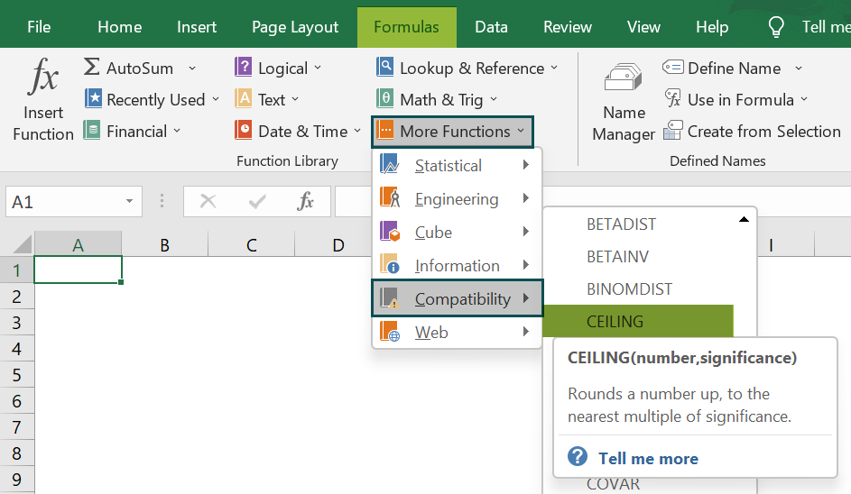
First, choose the cell for the output → select the “Formulas” tab → go to the “Function Library” → click the “More Functions…” drop-down → click the “Compatibility” option right arrow → select the “Ceiling” function, as shown below.

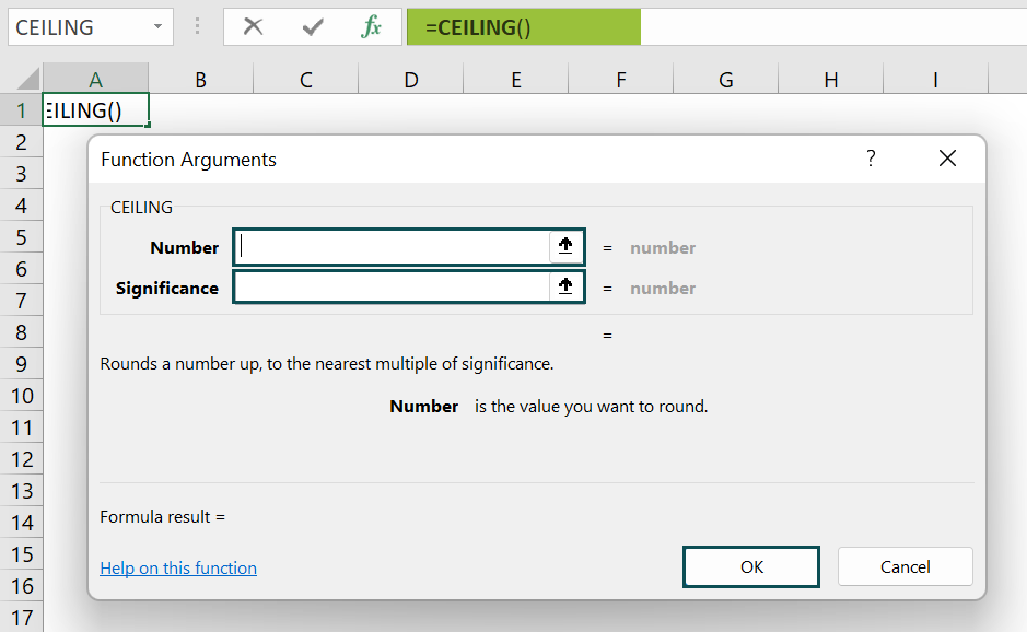
The “Function Arguments” window pops up. Enter the “Number” and “Significance” fields, as cell values or Excel cell references.

Method #2 – Enter in the Worksheet Manually

Select the cell for the output.
Type the formula =CEILING( in the selected cell. [Alternatively, type =C and double-click the CEILING() function from the Excel suggestions.]
Enter the number arguments in proper number format and the significance argument as values or cell references.
Close the brackets. Press the “Enter” key.

Let us take an example to explain this function. We will round off the Price Increase/Drop values using the Excel CEILING function.

The table below provides a list of items and the price increase and drops.

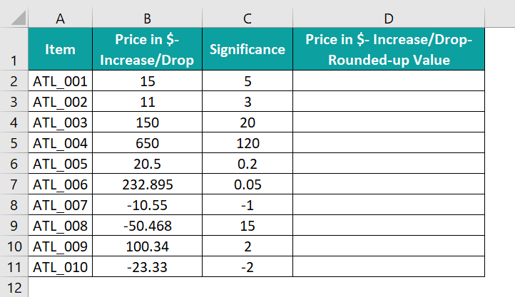
The steps to round the numeric values using the Excel CEILING function are:

Select cell D2, enter the formula =CEILING(B2,C2), and press the “Enter” key.

[Alternatively, select cell D2 and click Formulas → More Functions → Compatibility → CEILING to open the Function Arguments window.

The “Function Arguments” window opens.

Enter the values or cell references in the numbers and significance fields as shown below.

Click OK. We will get the required output in cell D2.]
Drag the formula from cell D2 to cell D11 using the fill handle.

The output is shown above.
[Note: We can directly enter the values as the function arguments instead of the cell references to the specific values. For example, the formula in the target cell D11 can also be: =CEILING(-23.33,-2)]

Examples

We will understand the Excel CEILING function with some advanced scenarios.

Example #1

We will see how the function works using the when the number argument is an Integer.

The following table shows stationery items as integers and their respective significance values.

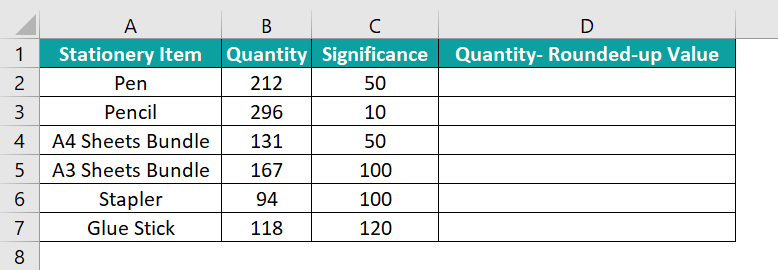
Step-by-Step procedure to round up the integer values using the Excel CEILING function are:

1: Select cell D2, enter the formula =CEILING(B2,C2), and press the “Enter” key.

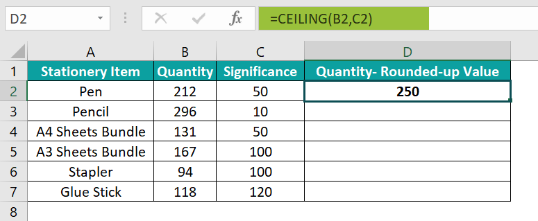
2: Drag the formula from cell D2 to D7 using the fill handle.

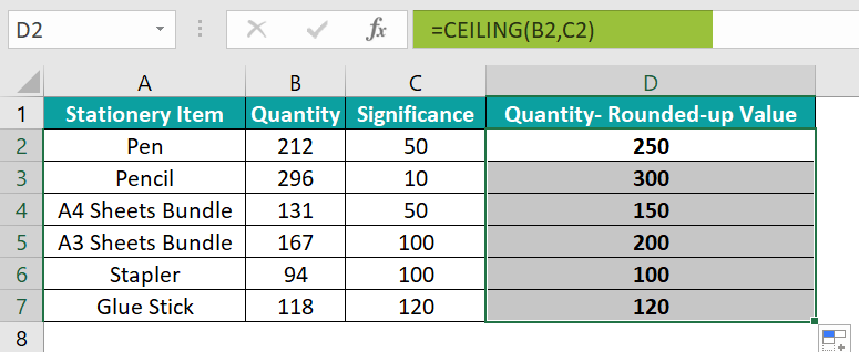
The output is shown above. The quantity values appear more presentable.

[Output Observation: Let us consider the first entry (Pen) to see how the CEILING() works. The number argument is 212, and the significance argument is 50. So, the multiples of 50 are 50, 100, 150, 200, 250, 300, and so on. And the nearest multiple of significance to which we can round up the number 212 is 250. Thus, the CEILING() output in cell D2 is 250.]

Example #2

We will see how the function behaves when the argument number is a fraction using the Excel CEILING function.

The following table shows a list of fruits and their quantity details.

Step-by-Step procedure to round up the fraction values using the Excel CEILING function are:

1: Select cell E2, enter the formula =CEILING(C2,D2), and press the “Enter” key.

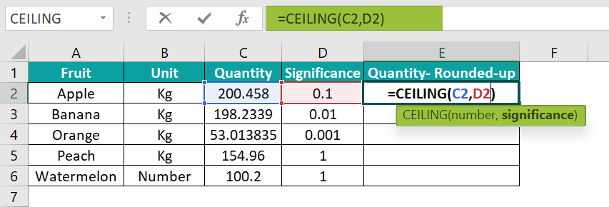
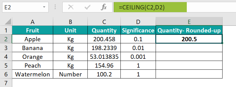
2: Drag the formula from cell E2 to E6 using the fill handle.

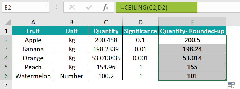
The output is shown above.

[Output Observation: When the number argument is a fraction, the CEILING() rounds up the value with the significance argument specifying the number of digits required after the decimal point.

For example, the quantity in cell C4 is 53.013835, and the corresponding significance value is 0.001. It implies we must round up the value 53.013835 to three decimal places. So, the immediate round-up value after 53.013 is 53.014, the CEILING function excel output in the target cell E4.

When the significance argument is 1, there are no digits after the decimal point. And as both arguments are positive, the round-up should be away from zero. So, the fraction gets rounded up to the immediate next integer value.]

Example #3

We can use the Excel CEILING function with other functions, such as ROW(), ISEVEN(), and ISODD(), and we can also use the conditional formatting feature to highlight the output.

The following table contains employees’ check-in and check-out times on a weekend.

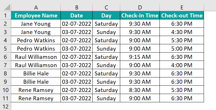
Step-by-Step procedure to use the CEILING function with ROW(), ISEVEN(), and ISODD() functions and conditional formatting are:

1: Select cell range A2:E11 → select the “Home” tab → go to the “Styles” group → click the “Conditional Formatting” drop-down → select the “New Rule” option to open the New Formatting Rule window.

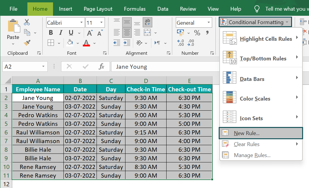
2: In the “New Formatting Rule” window,
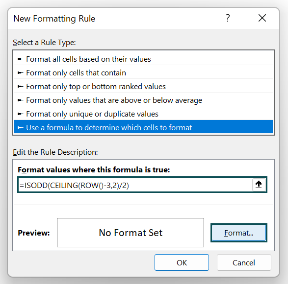
- Choose the “Use a formula to determine which cells to format” option in the “Select a Rule Type:” group.
- In the “Edit the Rule Description:” group, enter the formula =ISODD(CEILING(ROW()-3,2)/2) in the “Format values where this formula is true:” field.
- Click the “Format” button.

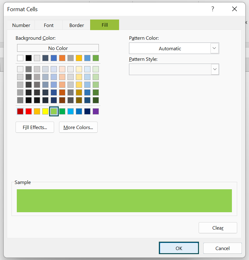
3: The “Format Cells” window opens. Now, click the “Fill” tab → go to the “Background Color” group → choose the required color from the color palette, here, “Green” → click “OK” to close the “Format Cells” window.

4: Click “OK” to close the “New Formatting Rule” window.

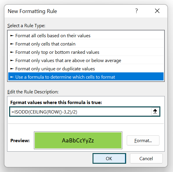
The output is shown below.

[Output Observation: Here is how the CEILING() formula works.

Consider the third row of the selected dataset (Row 4 – Pedro Watkins’s data). The ROW() will return the value 4. So the CEILING function becomes CEILING(4-3,2), that is, CEILING(1,2), which returns 2. Because 2 is the nearest multiple of significance, 2, the number 1 can get rounded up, using the CEILING().

Then, the ISODD function becomes ISODD(2/2), that is, ISODD(1), which returns TRUE. And so, row 4 gets shaded.]

Important Things To Note

The Excel CEILING function works for positive and negative numeric values. It rounds them up to a value away from 0.
If the arguments supplied to the CEILING() are non-numeric or cell references to non-numeric values, the function returns the #VALUE! error.
For a positive number and negative significance, the CEILING() output will be #NUM! error.
If the significance argument value is 0, the CEILING() will return the #DIV/0! Error.

Frequently Asked Questions (FAQs)

1. Where is the CEILING function in Excel?

The CEILING function in Excel is in the Formulas tab. Click Formulas → More Functions → Compatibility → CEILING to access it.

2. How to use the CEILING() in Excel VBA?

We can use the CEILING() in Excel VBA as follows:
The following table contains values for the two CEILING() arguments, number, and significance.

Step-by-Step procedure to update column C with the rounded-up numbers using the Excel CEILING function and VBA Macro are:

1: In the worksheet with the above table, press the keyboard shortcut Alt+F11 to open the VBA Editor window.

2: Choose the required VBA Project from the left menu in the VBA Editor window and click Insert → Module to open the Module1 window.

The module window opens, as shown below.

3: Enter the VBA code containing the CEILING function in the Module1 window, as shown in the image below.

Sub Ceiling_fn()
Dim rv As Worksheet
Set rv = Worksheets(“FAQ2”)
rv.Range(“C2”) = Application.WorksheetFunction.Ceiling_Math(rv.Range(“A2”), rv.Range(“B2”))
rv.Range(“C3”) = Application.WorksheetFunction.Ceiling_Math(rv.Range(“A3”), rv.Range(“B3”))
rv.Range(“C4”) = Application.WorksheetFunction.Ceiling_Math(rv.Range(“A4”), rv.Range(“B4”))
End Sub

4: Click the Run Sub/UserForm icon to run the code.

The output is shown below. Once we run the code, the rounded-up values generate in the target cells.

[Note: The CEILING.MATH() replaced CEILING() in Excel version 2013. So, the VBA code uses the “Application.WorksheetFunction.Ceiling_Math()” to round up the values.]

3. Why is the CEILING function not working in Excel?

A few reasons the CEILING function is not working in Excel are:
· The supplied CEILING() arguments are non-numeric.
· One of the arguments, i.e., the significance argument, maybe 0.
· The number argument is positive, and the significance argument is negative.

4. What is the use of the CEILING function in Excel?

The use of the CEILING function in Excel is that it rounds up the given numeric value to the immediate next multiple of the specified significance.
For example, we can set up the price values after currency conversions.

Download Template

This article must help understand the Excel CEILING function, with its formula and examples. We can download the template here to use it instantly.

Excel CEILING Function Download

Excel CEILING Function