What Is Freeze Cells In Excel?
Freeze cells in Excel refer to a useful feature that allows users to maintain specified rows or columns visible on their screen while scrolling through large data sets. We can keep important information visible by freezing cells, ensuring easy reference or comparison without continuous manual scrolling. This feature proves particularly beneficial when working with extensive spreadsheets containing headers, labels, or other crucial information that may otherwise become hidden as we navigate the document.
Freeze cells enable professionals to swiftly analyze and manipulate data while keeping pertinent details readily accessible. Particularly efficient for long lists or complex datasets, freezing cells in Excel promotes increased productivity and accuracy by minimizing time spent searching for essential information during data exploration or analysis tasks.
📥Download the ready-to-use Excel template to practice this tutorial yourself.
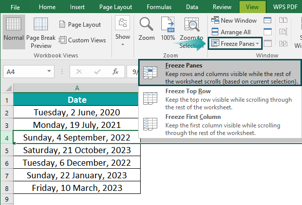
Freeze-Cells-in-ExcelBelow is a simple example illustrating how to freeze rows in a spreadsheet.
Step 1: Start by clicking on the corresponding row number to freeze a specific row.
Step 2: Next, navigate to the View tab located on the ribbon.
Step 3: From there, select the Freeze Panes command.

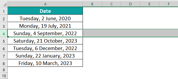
A subtle gray line indicates that the selected rows will remain fixed in position. This allows us to scroll through the worksheet effortlessly while keeping the frozen rows visible at the top.

Table of contents
Key Takeaways
- Freeze Panes in Excel feature freezes the cells such that they appear throughout the worksheet.
- One of the primary purposes of freezing cells in Excel is to facilitate easy viewing and data analysis, particularly when dealing with large or complex datasets.
- To quickly access the “Freezing Panes” command, press the “ALT + W + F” shortcut keys to freeze and unfreeze panes as needed, streamlining our workflow.
- Also, it offers a valuable functionality called “Print Titles,” specifically designed for printing spreadsheets.
How To Freeze Cells In Excel?
Freezing cells in Excel can be a useful tool for managing large amounts of data and improving the readability of worksheets.
- To freeze cells, select the row below and the column to the right where we want to freeze.
- Next, navigate to the View tab on the Excel ribbon and click Freeze Panes.
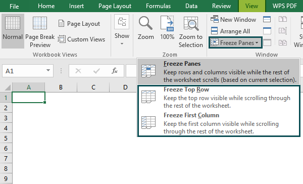
- A drop-down menu will appear with three options: Freeze Panes, Freeze Top Row, and Freeze First Column.
- Select the appropriate option based on our needs. If we want to freeze rows and columns, choose Freeze Panes in excel.
- This will lock the selected rows and columns into place while allowing us to scroll freely through other areas of our worksheet.
- By freezing cells in this manner, important headers or labels can remain visible at all times, making it easier to work with extensive datasets or compare information across different spreadsheet sections.
Examples
Example #1
Below is an example of how to freeze rows.
Step 1: To freeze a specific row, begin by clicking on the corresponding row number.
Step 2: Next, navigate to the View tab on the ribbon. From there, select the Freeze Panes command.

Step 3: Once frozen, the selected rows will remain in place, indicated by a gray line. We can freely scroll through the worksheet while viewing the frozen rows at the top. Refer to the snapshot below to see the frozen rows above the gray line that remain fixed even when scrolling.

Step 4: To unfreeze the cells, follow the same process. After freezing the cells, the View tab will display the Unfreeze Panes command instead of Freeze Panes in Excel. By clicking on this command, the frozen cells will be unfrozen, allowing us to scroll through all rows and columns in the worksheet.

Example #2
Below is a straightforward example of how to freeze cells in Excel.
Step 1: To freeze columns, click on the alphabet corresponding to the desired column.
Step 2: Go to the View tab on the excel ribbon. From there, choose the Freeze Panes command.

Step 3: The selected columns will now be frozen, indicated by a gray line. We can freely scroll through the worksheet while still viewing the frozen columns. The snapshot below shows that the columns adjacent to the gray line remain fixed even when scrolling.

Step 4: To unfreeze the columns, follow the same process used for unfreezing rows by selecting the Unfreeze Panes command in the View tab. Additionally, there are two other options within the Freeze Panes menu: Freeze Top Row and Freeze First Column.

These commands specifically freeze the top row and the first column, respectively. For instance, the Freeze Top Row command locks row number 1, while the Freeze First Column command locks the cell in column A. It’s worth noting that we can also freeze rows and columns simultaneously. Furthermore, locking only one row or column at a time is not mandatory.

Use Of Rows & Column Freezing In Excel Cell
Rows and column freezing in Excel cell is a powerful feature that enables professionals to navigate through large datasets and complex spreadsheets effortlessly. By freezing specific rows or columns, users can ensure that important headings or reference data are always visible as they scroll vertically or horizontally. This functionality is especially valuable when analyzing financial statements, conducting data analysis, or preparing reports. Professionals can select the row beneath their desired frozen row or the column to the right of their chosen frozen column, ensuring the crucial information remains fixed. At the same time, they explore other parts of the spreadsheet. By constantly eliminating the need to move back and forth within a large dataset, rows and column freezing allows professionals to focus on interpreting data accurately and making informed decisions efficiently. This simple yet effective feature greatly enhances productivity, enabling professionals to navigate complex spreadsheets with ease and precision effortlessly.
Important Things To Note
- After activating the Frozen Panes command in an Excel worksheet, pressing the CTRL + Home shortcut keys no longer position the cell cursor in cell A1.
- Instead, Excel places the cursor in the first unfrozen cell, providing a more efficient navigation experience.
- When freezing both rows and columns in Excel, selecting the cell above the desired frozen area is essential. This selection method eliminates the need to choose the entire row and column simultaneously.

Frequently Asked Questions (FAQs)
• Excel allows users to freeze rows and columns to remain visible while scrolling through a large dataset.
• Another limitation of freezing cells is that it restricts the ability to perform certain actions, such as sorting data or creating pivot tables. Freezing panes can also cause issues with printing, as the frozen rows or columns may repeat on every printed page, leading to unnecessary duplication of information.
The main difference between these two features lies in how they control visibility and scrolling within an Excel spreadsheet.
Below is a simple example demonstrating how to freeze Excel cells. To freeze columns, click on the alphabet corresponding to the desired column. Once the columns are selected, navigate to the View tab on the ribbon. From there, choose the Freeze Panes command.
As a result, the selected columns will be frozen, clearly indicated by a distinct gray line. This allows us to effortlessly scroll through the worksheet while still viewing the frozen columns.
To split the selected column, press the Split button. This action will result in the spreadsheet being divided into two sections, with the selected cells as the splitting point.
• The purpose of freezing cells is to ensure selected rows or columns remain visible by freezing cells.
• It is important to freeze while working with extensive worksheets containing numerous rows and columns, enabling professionals to comprehend data relationships and make accurate comparisons without losing sight of vital information.
• Freezing cells also proves beneficial when creating reports or conducting analyses requiring constant reference to specific headers or labels.
Download Template
📥Download the ready-to-use Excel template to practice this tutorial yourself.
Freeze-Cells-in-ExcelRecommended Articles
Guide to Freeze Cells in Excel. Here we learn how to freeze cells in excel with step by step examples and template. You can learn more from the following articles –

Leave a Reply