Inverse Matrix in Excel

What is Inverse Matrix in Excel?

An inverse matrix in Excel can be determined using the MINVERSE function. It is not easy to determine the inverse of a singular matrix. However, using the MINVERSE function, we can find the inverse of a matrix containing the same number of rows and columns.

The inverse of a matrix means the reciprocal of a square matrix whose determinant is not equal to zero. Here, a square matrix has an equal number of rows and columns.

For instance, let us consider a 3*3 matrix in cells B2 to D4. To find the inverse of this matrix, you must highlight a matrix equal in dimension to the one you want to reverse. Here, we highlight cells F2 to H4 since we want to find the inverse for a 3*3 matrix. Once highlighted, type =MINVERSE( in cell F2, the first cell of the matrix. Next, select the cells from B2 to D4 as the cell range. The function becomes =MINVERSE(B2:D4). Now, simultaneously press Control + Shift + Enter because it is an array formula in excel. You get the resultant inverse matrix in cells F2 to H4.

What is Inverse Matrix in Excel?

The MINVERSE function is used to find the inverse matrix in Excel. It can be used for any square matrix containing an equal number of rows and columns.
MINVERSE takes a single argument, which can be specified as a cell range or an array constant like {1,2;2,4}.
You can determine the inverse of matrices whose determinants are not zero. Also, an identity matrix is a product of a matrix and its inverse. Only the diagonal is one, and the remaining elements are zero.

Inverse Matrix – Explanation and Uses

The Inverse matrix in Excel provides the reciprocal of any square matrix. We have to use the function MINVERSE in Excel to find the inverse of a matrix. The syntax of the formula is as follows:

Inverse Matrix in Excel - MINVERSE formula

Here, the array could be a cell range or an array constant.

You must select the output range and enter the formula in its leftmost top cell to get the output.
Then, press CTRL+SHIFT+ENTER to make it an array formula. Curly brackets are inserted at the beginning and end of the formula.
It is done for all versions except the current version of Microsoft 365.

Uses

The application of the inverse matrix is as follows:

We can use the inverse matrix to solve linear equations.
Inverse matrices are used to solve mathematical equations where several variables are used.
Programmers use inverse matrices in the encryption of messages.
Matrix computations like inverse are used to calculate electrical circuits, networking, quantum mechanics, etc. The inverse matrix is used in measuring battery power outputs.
Inverse matrices are used in input and output analysis in economics.

How to Use Inverse Matrix in Excel?

We can solve inverse matrix in Excel in two ways.

Entering MINVERSE() manually in Excel
Access from the Excel ribbon.

Method #1 – Entering MINVERSE() Manually in Excel

Let us look at how we can manually enter the function MINVERSE to determine the inverse matrix in Excel.

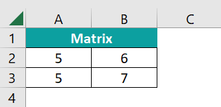
First, enter the matrix whose inverse we must determine in the Excel sheet. Here, we enter a 2*2 matrix in the cells A2 to B3.
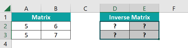
Next, to get the result, select the same area as that of the matrix. For example, since we are finding the inverse of a 2*2 matrix, select the cells D2 to E3 to get the result of the 2*2 matrix.
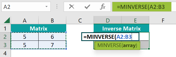
Now, type =MINVERSE( in the formula bar. Select the matrix area from A2 to B3.
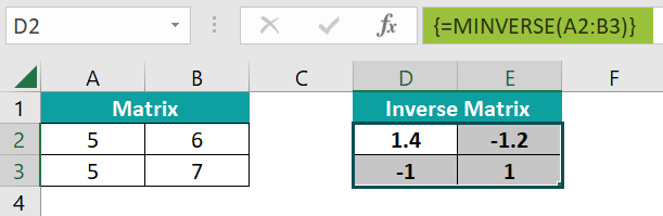
Press Ctrl + Shift + Enter. The formula gets converted into an array formula with curly braces. {}. Thus, you get the inverse of the matrix in D2:E3 by manually entering MINVERSE in Excel.

Method #2 – Access from the Excel Ribbon

Step 1: Choose any cell and go to the “Formulas” tab. Here, go to the “Function Library” group, and click on the “Math & Trig” drop-down arrow. Choose the MINVERSE function.

Inverse Matrix in Excel - Access from the Excel ribbon - Step 1

Step 2: In the popup window, enter the array whose matrix we must find, as shown below with curly braces; a semi-colon separates each row. Press OK.

Inverse Matrix in Excel - Access from the Excel ribbon - Step 2

Step 3: Thus, you get the inverse matrix by entering MINVERSE through the Excel ribbon.

Inverse Matrix in Excel - Access from the Excel ribbon - Step 3

Examples

Now that we have seen how to find the inverse matrix with an example let us try applying the same in a few examples to find the inverse matrix in Excel.

Example #1

To begin with, we create inverse matrix in Excel as below. Then, let us determine the inverse of a 3*3 matrix, as shown below.

Step 1: To find the inverse of A, we must use the MINVERSE excel function. Select an area equal to the size of matrix A. Here, we select F2 to H4. Now, go to the formula bar and type =MINVERSE(

Step 2: Select the array from B2 to D4. Close the braces.

Step 3: Press Ctrl + Shift + Enter. Now you get the inverse of the Matrix A in cells F2 to H4.

Inverse Matrix in Excel - Example 1 - Step 3

Finding the matrix using the MINVERSE function is simple and reduces the effort and time spent on complex calculations.

Example #2

Let us take another example to find inverse matrix in Excel. We have a 3*3 matrix, A. We must find the inverse matrix in Excel for A.

Step 1: Select a 3*3 array equal to the dimension of matrix A. Here, we select cells F2 to H4. Enter the formula as =MINVERSE( and select the array from B2 to D4.

Step 2: Close the braces and press Ctrl + Shift + Enter. You get the value of A^-1.

Inverse Matrix in Excel - Example 2 - Step 2

Step 3: Now, we can verify the result by multiplying A with A^-1.The resultant matrix is called a unit or identity matrix of the form.

Select the cells equal to the 3*3 matrix. Here we select D8 to F10.
Enter the formula as =MMULT(B2:D4,F2:H4).
Press Ctrl + Shift + Enter.

Inverse Matrix in Excel - Example 2 - Step 3

We get the identity matrix as seen, proving that our inverse matrix result is accurate.

Example #3

Let us look at how we can apply the inverse matrix solution in a real-life example. A group of adults and children go to a circus. The tickets are priced at $5 per child and $ 7 per adult. The total amount spent was $215. Afterwards, they went to a fair where the tickets were priced at $4.50 and $6 for children and adults, respectively. Here, the total amount spent was $189. Find the number of children and adults here.

Step 1: For this, we build two matrices, as shown below.

Excel Inverse Matrix - Example 3 - Step 1

Step 2: The resultant matrix of these two is in cells H2 and I2.

Step 3: The above matrices are of the form AX = B. To solve for X, we must multiply the equation by A^-1. So, to get the number of children and adults, we must solve the equation,

X = BA^-1

To find the inverse of A, select the cells of the same size as Matrix A. For example, we choose E7 to F8 since it is a 2*2 matrix.

Go to the formula bar, type =MINVERSE(.
Select the matrix A array from E3 to F4.

Step 4: Press Ctrl + Shift + Enter after closing the braces. You get the inverse of matrix A in E7 to F8.

Inverse Matrix in Excel - Example 3 - Step 4

Step 5: Using the MMULT function, multiply matrix B with the inverse of A. Here the resultant will be a 1*2 matrix. So, select cells H7 and I8.

Go to the formula bar and type =MMULT(.
Select the matrix B from H3 to I3 and the A^-1 array from E7 to F8.

Step 6: Close the braces and press Ctrl + Shift + Enter.

Inverse Matrix in Excel - Example 3 - Step 6

Thus, you get the answers in the resultant matrix, which indicates the number of children as 15 and the number of adults as 22.

Important Things to Note

We must enter MINVERSE as an array formula. For this, in Excel 2003 or later versions, you must press Ctrl + Shift + Enter, except in Microsoft 365.
You get the #VALUE error while using the MINVERSE function when the matrix contains non-numerical values, a different number of rows and columns, or empty cells.
You can verify the result of your inverse matrix by multiplying the original matrix with the inverse. If you get an identity matrix, your result is accurate.
#N/A error is obtained when the cells of the inverse matrix are out of range.
You get an #NUM error if you can’t get the matrix inverse.

Frequently Asked Questions (FAQs)

1. Why is inverse matrix in Excel not working?

You get an error for the inverse matrix in Excel under the following conditions:
• The MINVERSE formula should be entered as an array formula for it to work. You must enter the formula and then press CTRL + SHIFT + ENTER.
• You get an #VALUE error when your array elements are non-numerical or if the matrix is not a square.
• You get an #NUM error if the determinant of the matrix is zero.

2. What is the use of inverse matrix in Excel?

The primary use of the inverse matrix in Excel is to solve the system of linear equations. However, it is also used in various fields which require matrix computations, such as electric circuits, quantum mechanics, airplanes, and spacecraft.

3. What are the requirements for inverse matrix in Excel?

The main requirements for the inverse matrix are as follows:
• It should be a square matrix with an equal number of rows and columns.
• It should not be a singular matrix, that is, the determinant should not be zero.
• No cells should be empty or non-numeric in the matrix.

Download Template

This article must help understand the Inverse Matrix in Excel, with its formula and examples. You can download the template here to use it instantly.

Inverse Matrix in Excel Download