1. How to multiply a 3x1 matrix with a 1x3 matrix using the MMULT function in Excel?

You can multiply a 3x1 matrix with a 1x3 matrix using the MMULT function in Excel in the following way. Let us see the steps with an example. The below image shows two arrays under Input Data. While the first array is a 3x1 array, the second one is a 1x3 array. Thus, multiplying the two given arrays results in a 3x3 matrix. And here is how the MMULT function can help you get the required matrix product in the target cell range B12:D14. • Step 1: First, select the target cell range B12:D14 and then, enter the MMULT() formula. =MMULT(B6:B8,D6:F6) • Step 2: Next, press the Ctrl + Shift + Enter keys to execute the above formula as an array formula. {=MMULT(B6:B8,D6:F6)}

MMULT In Excel

What Is MMULT Function In Excel?

The MMULT function in Excel is an inbuilt Math & Trig function that calculates the matrix product of the two supplied arrays. The function output will be an array with the number of rows and columns as same as array1 and array2, respectively. Users can utilize the function MMULT in Excel when they have to multiply parameters given in matrix form and require the product in the matrix form.

For example, the below image shows two 2×2 arrays, Array 1 and Array 2.

And suppose the requirement is to multiply the two given matrices and display the resulting product in the cell range A11:B12, then using MMULT in Excel in the cell range A11:B12, we can get the required data.

In the above MMULT in Excel example, as the number of rows in the first array is two and the number of columns in the second array is 2, their product is a 2×2 array.

What Is MMULT Function In Excel?

The function MMULT in Excel multiplies the two given arrays.
The MMULT() accepts two mandatory arguments, array1 and array2, as inputs.
In case of Office 365, we can enter the MMULT() in the top-left cell of the target cell range and press Enter to apply the formula as a dynamic array formula. However, when using the previous Excel versions, we can select the required cell range and enter the MMULT().
But while executing the function, press the Ctrl + Shift + Enter keys to apply it as an array formula.

MMULT() Excel Formula

The syntax of MMULT Formula in Excel is:

where,

array1: The first matrix values.
array2: The second matrix values.

The two arguments in the MMULT Formula in Excel are mandatory.

Please Note: If you use the Office 365 version, you can enter the MMULT() formula in the top-left cell of the output cell range. And then, you can press Enter to execute the formula as a dynamic array formula.

However, if we use Excel 2019 or previous versions, we can select the target cell range and enter the MMULT() formula. And then, we should execute it as an array Excel formula using the Ctrl + Shift + Enter keys.

Further, if the function MMULT in Excel returns error, we can check the below points to identify the root cause.

The two given arrays should have only numbers.
The number of columns in array1 and rows in array2 should be the same.
We can supply array1 and array2 as cell ranges, Excel cell references, or array constants.
The function MMULT in Excel returns error #VALUE! when:
- The given arrays contain empty cells, or the cell values are texts.
- The number of columns in array1 and rows in array2 is different.

Excel VBA – All in One Courses Bundle (35+ Hours of Video Tutorials)

If you want to learn Excel and VBA professionally, then Excel VBA All in One Courses Bundle (35+ hours) is the perfect solution. Whether you’re a beginner or an experienced user, this bundle covers it all – from Basic Excel to Advanced Excel, Macros, Power Query, and VBA.

Start Learning Now

How to Use MMULT Excel Function?

The steps to use the function MMULT in Excel are as follows:

First, ensure the two supplied matrices contain only numbers. Also, confirm that the number of columns in array1 and the number of rows in array2 are the same.
Then, select the target cell range, where we need to display the matrix product of the two given arrays and enter the function MMULT().
Finally, press the keys Ctrl + Shift + Enter to execute the function MMULT in Excel as an array formula.

Here is an example that explains the MMULT in Excel definition and the above steps to apply the function properly.

The following image shows two 3×3 arrays, Array 1 and Array 2.

Suppose we need to find the matrix product of the two arrays and display the result in the cell range B11:D13. Then using MMULT in Excel function in the cell range B11:D13 is a straightforward way to achieve the desired data.

To begin with, select the target cell range B11:D13 and enter the MMULT() formula.
=MMULT(B6:D8,F6:H8)
Next, press the Ctrl + Shift + Enter keys to apply the MMULT() in the target cell range as an array formula.
{=MMULT(B6:D8,F6:H8)}

We can also supply the numbers in the two arrays directly as the MMULT() arguments to get the above-resulting matrix.
=MMULT({1,2,3;4,5,6;7,8,9},{10,100,1000;100,1000,10;1000,10,100})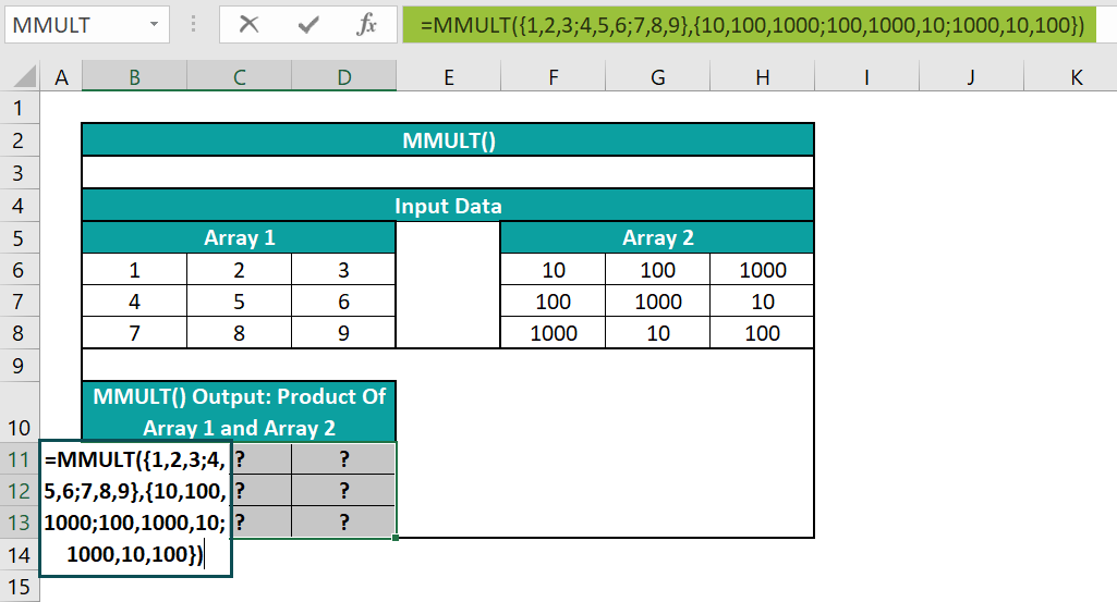

We can then press the Ctrl + Shift + Enter keys to apply the MMULT() in the target cell range as an array formula to get the required product value.

Alternatively, we can apply the MMULT() using the option available in the Formulas tab. And for that, we need to select the required target cell range, B11:D13, and click Formulas → Math & Trig → MMULT to open the Function Arguments window.

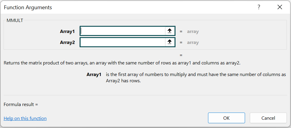
Next, enter the two given array ranges as Array1 and Array2 field values in the Function Arguments window.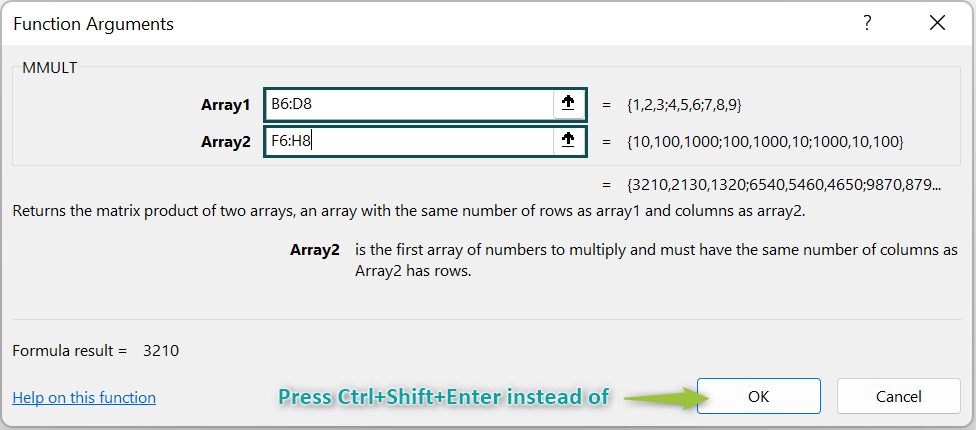

Finally, press the Ctrl + Shift + Enter keys instead of clicking OK in the Function Arguments window to apply the MMULT() as an array formula.

Let us see how the MMULT() works in the target cell B11. The formula in cell B11 will be:
=1*10 + 2*100 + 3*1000
= 10 + 200 + 3000
=3210

Examples

Check out the following examples to understand the MMULT in Excel definition more effectively.

Example #1

The mathematical representation of the matrix product array c of two given arrays, a,and b, is:

where,

a and b: The two given arrays (matrices).
c: The resulting matrix product of the two given arrays.
i: The row number.
j: The column number.

Let us take two 2×2 matrices and solve the above equation to find their product. The outcome will be the same as when applying the function MMULT in Excel with the two 2×2 matrices supplied as the Function Arguments.

The below image shows two arrays, a and b.

If we have to find the product of the two given arrays, the result will also be an array, like, c.

Then, we can perform the required mathematical evaluation using the equation provided above or apply the function MMULT in Excel in the target cell range.

Step 1: Select the target cell C11, enter the below formula, and press Enter.

=C4*F4+D4*F5

Here, the value of the variables i and j is one, and the variable k is two, as the resulting array is a 2×2 matrix. So, the cell C11 value is c₁₁, and the equation in cell C11 becomes:

c₁₁ = a₁₁ * b₁₁ + a₁₂ * b₂₁

= 4*11 + 8*12

= 44 + 96

= 140

Likewise, enter the respective equations in cells D11, C12, and D12.

The mathematical equation in cell D11:

c₁₂ = a₁₁ * b₁₂ + a₁₂ * b₂₂

The mathematical equation in cell C12:

c₂₁ = a₂₁ * b₁₁ + a₂₂ * b₂₁

The mathematical equation in cell D12:

c₂₂ = a₂₁ * b₁₂ + a₂₂ * b₂₂

Step 2: Select the target cell range F11:G12 and enter the MMULT().

=MMULT(C4:D5,F4:G5)

Next, press the keys Ctrl + Shift + Enter to execute the function as an array formula.

{=MMULT(C4:D5,F4:G5)}

Thus, now we know how the MMULT() calculates the product values.

Example #2

In this MMULT in Excel example, we shall see how to apply the function in a real-world scenario.

The following image shows two arrays. The first matrix contains the sports balls’ quantity data for January and February. And the second matrix contains the weight and price data for the specified sports balls.

Suppose the requirement is to determine the total weight and price for the required quantities of the sports balls in January and February and display the output in the cell range B9:C10.

While the first array is a 2×3 matrix (B3:D4), the second array is a 3×2 matrix (G3:H5). So, as the number of columns in the first array is the same as the number of rows in the second array, we can find the product of the two given arrays to get the required output. And since the first array row count and the second array column count form the number of rows and columns for the resulting matrix, the output will be a 2×2 array.

Step 1: First, select the target cell range B9:B10 and enter the function MMULT in Excel.

=MMULT(B3:D4,G3:H5)

Step 2: Next, press the Ctrl + Shift + Enter keys to execute the function MMULT in Excel as an array formula.

{=MMULT(B3:D4,G3:H5)}

Example #3

We can apply the function MMULT in Excel to count the number of rows in a cell range containing a specific value.

However, the given value may appear in more than one column. Thus, we can use the MMULT() with COLUMN, TRANSPOSE, and SUM Excel function to count such instances of the specific value as one and resolve the issue.

For example, the below table contains four arrays, Array A, Array B, Array C, and Array D.

Suppose we need to determine the number of rows in the above table containing the value 20 and display the result in cell E13. Then here is how we can achieve the required count using the function MMULT in Excel with the functions SUM, TRANSPOSE, and COLUMN in the target cell.

Step 1: To begin with, select the target cell E13, and enter the below formula.

=SUM(–(MMULT(–(A2:D11=20),TRANSPOSE(COLUMN(A2:D11)))>0))

Step 2: Next, press the Ctrl + Shift + Enter keys to execute the above formula as an array formula.

{=SUM(–(MMULT(–(A2:D11=20),TRANSPOSE(COLUMN(A2:D11)))>0))}

Explanation

First, the term (A2:D11=20) shows the cells containing the value 20 as TRUE and the remaining as FALSE.
Then the double negation operator converts the TRUE and FALSE values into 1 and 0, thus resulting in a 10×4 array.
Next, the COLUMN() returns the column numbers in the range A2:D11, which the TRANSPOSE() changes into row numbers, thus giving a 4×1 array.
Next, the MMULT() finds the product of the two 10×4 and 4×1 matrices, returning a 10×1 matrix {3;1;0;7;0;2;0;1;2;0}. And once these values get compared to 0, the values greater than 0 become TRUE, and the remaining values become FALSE.
The double negation operator converts the TRUE and FALSE values into 1 and 0.
And finally, the SUM() adds all the 1s to return the value 6, the number of rows containing the value of 20.

Please Note: The value 20 appears twice in row 5. But the above formula counts it as only one occurrence, as the value is in the same row but more than one column.

Important Things To Note

We can apply the function MMULT in Excel only when the two given arrays which we need to multiply contain numbers.
Ensure the number of columns in array1 and rows in array2 is the same.
The arguments array1 and array2 can be cell ranges, references, or array constants.
Suppose the supplied arrays contain blank cells or text values, or the number of columns in array1 and rows in array2 are not the same. Then the MMULT() returns the #VALUE! error.

Frequently Asked Questions (FAQs)

1. How to multiply a 3×1 matrix with a 1×3 matrix using the MMULT function in Excel?

You can multiply a 3×1 matrix with a 1×3 matrix using the MMULT function in Excel in the following way. Let us see the steps with an example.

The below image shows two arrays under Input Data.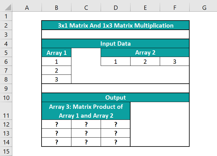

While the first array is a 3×1 array, the second one is a 1×3 array. Thus, multiplying the two given arrays results in a 3×3 matrix.

And here is how the MMULT function can help you get the required matrix product in the target cell range B12:D14.

• Step 1: First, select the target cell range B12:D14 and then, enter the MMULT() formula.
=MMULT(B6:B8,D6:F6)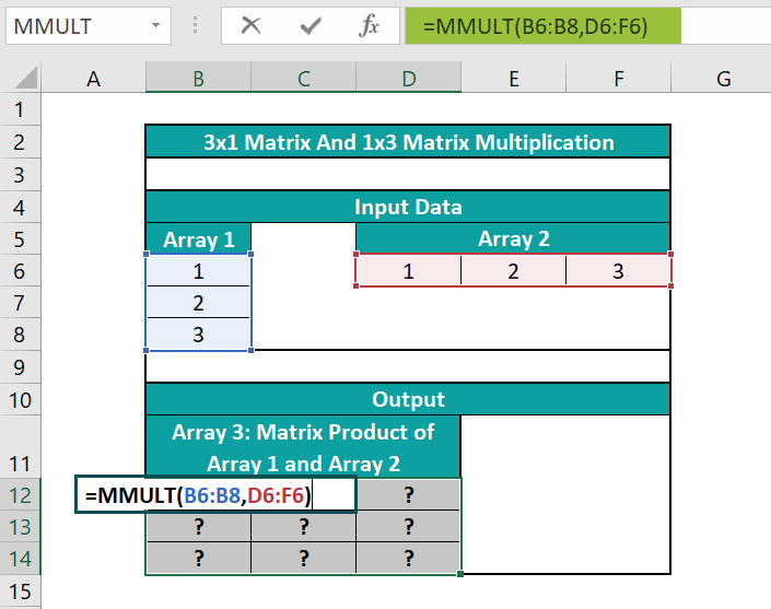

• Step 2: Next, press the Ctrl + Shift + Enter keys to execute the above formula as an array formula.
{=MMULT(B6:B8,D6:F6)}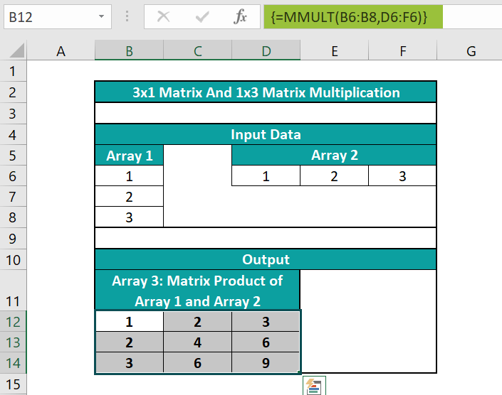

2. How to apply the MMULT function in Excel VBA?

You can apply the MMULT function in Excel VBA using the method:

Application.WorksheetFunction.MMult(array1,array2)

The function arguments are the two input arrays you must multiply to get the matrix product.

3. Why is the MMULT in Excel not working?

The MMULT in Excel is not working, perhaps because of the following reasons:
• The supplied arrays contain empty cells or text values.
• The number of columns in array1 does not equal the number of rows in array2.
• The target cell range you choose to show the resulting matrix exceeds the required range.

Download Template

This article must be helpful to understand the MMULT In Excel, with its formula and examples. You can download the template here to use it instantly.

MMULT In Excel Download

MMULT In Excel