COLUMNS Function in Excel

What Is COLUMNS Function In Excel?

The COLUMNS Function in Excel calculates the number of columns in the given array. The function is used to know the number of columns in an array of references.

The COLUMNS Function in Excel is categorized under the Lookup & Reference group of the functional library of the formula tab.

For example, the image below depicts the values, and we will calculate the total number of columns in a range using the COLUMNS functions in Excel.

The steps to calculate the number of columns by the COLUMNS Function in Excel are as follows:

Step 1: First, select the column where we will enter the formula and then, calculate the result. In this example, we have selected cell C2.

Step 2: Next, we will enter the Excel COLUMNS Formula in cell C2.

Step 3: Then, enter the value of the array argument as A1:B2, i.e., the range of columns.

Step 4: Now, the complete formula entered is =COLUMNS(A1:B2).

Step 5: Next, press Enter key.

We can see the results in cell C2.

Likewise, we can use columns function in excel to obtain the results.

What Is COLUMNS Function In Excel?

The COLUMN function returns the column number of the given cell reference.
The syntax of the COLUMN function is =COLUMN([reference]).
The reference argument could not refer to multiple areas.
If we do not enter the argument value, the function will automatically refer to the cell that contains the COLUMN formula.
An array is a range or contiguous group of cells.
The ROW function counts the number of rows.
Similarly, the COLUMN function counts the number of columns and it always returns a numeric value.

Syntax

array = This is the mandatory argument. This refers to a range of cells with which the number of columns is calculated.

Excel VBA – All in One Courses Bundle (35+ Hours of Video Tutorials)

If you want to learn Excel and VBA professionally, then Excel VBA All in One Courses Bundle (35+ hours) is the perfect solution. Whether you’re a beginner or an experienced user, this bundle covers it all – from Basic Excel to Advanced Excel, Macros, Power Query, and VBA.

Start Learning Now

How To Use COLUMNS Formula In Excel?

1. Access From The Excel Ribbon

To begin with, choose the empty cell which will contain the result.
Then, go to the Formulas tab and then, click it.
Next, select the Lookup & Reference option from the menu.
Finally, choose COLUMNS from the drop-down menu.

How to use COLUMNS Function in Excel - Access from the Excel ribbon

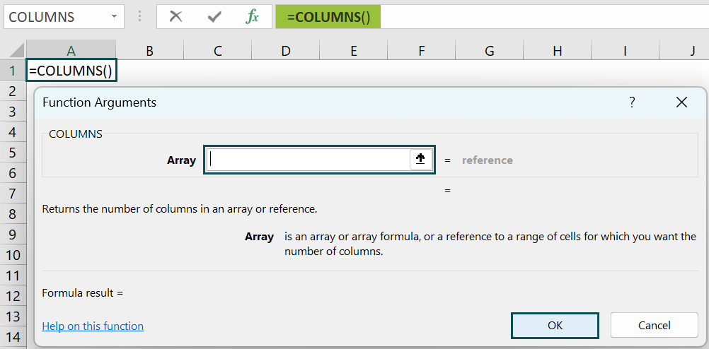
A window called Function Arguments appears.
Next, enter the value in the array.
Then, select OK.

How to use COLUMNS Function in Excel - Function arguments window

2. Enter The Worksheet Manually

To start with, select an empty cell for the output.
Next, type =COLUMNS( in the selected cell. Alternatively, type =C and double-click the COLUMNS function from the list of suggestions Excel shows.
Finally, press Enter key.

Examples

Example #1 – Total Columns In A Range

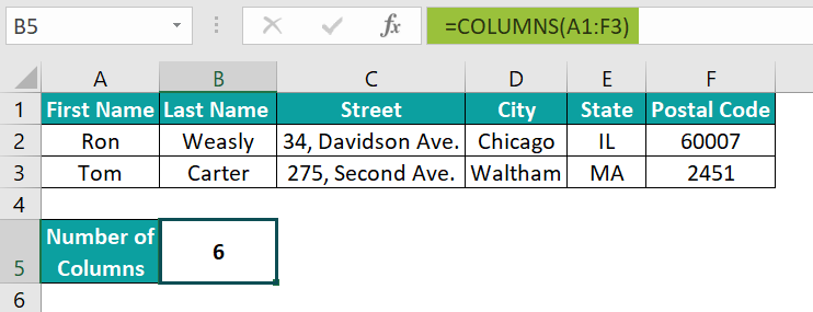
The following example depicts the name and addresses of people, and we will calculate the total number of columns in a range using the COLUMNS functions in Excel.

In the table,

Column A, B, C, D, E, and F contains the first name, last name, street, city, state and postal code respectively.
We need to find the number of columns in row 5.

COLUMNS Function in Excel - Example 1 - Total Columns in a Range

The steps to calculate the number of columns by the COLUMNS Function in Excel are as follows:

Step 1: First, select the column where we will enter the formula and calculate the result. The selected cell, in this case, is cell B5.

Step 2: Next, we will enter the Excel COLUMNS Formula in cell B5.

Step 3: Then, enter the value of the array argument as A1:F3, i.e., the range of columns.

Step 4: Now, the complete formula entered is =COLUMNS(A1:F3).

Example 1 - Total Columns in a Range - Step 4

Step 5: Press Enter key.

We can see the results in cell B5 as 6.

Example 1 - Total Columns in a Range - Step 5

Similarly, we can find the number of columns using columns function in excel.

Example #2 – Total Cells In A Range

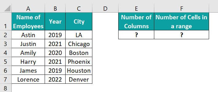
The following example depicts the name and people’s employment details, and we will calculate the total number of cells in a range using the COLUMNS functions with the ROWS function in Excel.

In the table,

Column A, B, C, D, E, and F contains the name of employees, year of joining, city, number of columns and number of cells in a range.
Row 3 contains the Formula.

COLUMNS Function in Excel - Example 2 - Total Cells in a Range

The steps to calculate the number of columns by the COLUMNS Function in Excel are as follows:

Step 1: To begin with, select the column where we will enter the formula and then, calculate the result of the total number of columns. The selected cell, in this case, is cell E2.

Step 2: Next, we will enter the Excel COLUMNS Formula in cell E2.

Step 3: Then, enter the value of the array argument as A1:C7, i.e., the range of columns.

Step 4: The complete formula entered is =COLUMNS(A1:C7).

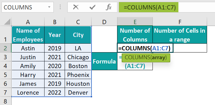
Example 2 - Total Cells in a Range - Step 4

Step 5: Now, press Enter key. The result is obtained in cell E2 as 3.

Example 2 - Total Cells in a Range - Step 5

Step 6: Select the column where we will enter the formula and calculate the result of the total number of cells. The selected cell, in this case, is cell F2.

Step 7: Next, we will enter the Excel COLUMNS Formula and ROWS formula in cell F2.

Step 8: Enter the value of the array argument as A1:C7, i.e., the range of columns.

Step 9: Similarly, enter the value of the array argument as A1:C7, i.e., the range of rows.

Step 10: The complete formula entered is =COLUMNS(A1:C7) * ROWS(A1:C7).

Example 2 - Total Cells in a Range - Step 10

Step 11: Next, press Enter key. The result is derived in cell F2 as shown in the image below.

Example 2 - Total Cells in a Range - Step 11

Example #3 – Get The Address Of The First Cell In A Range

The following example depicts the region-wise monthly sales, and we will calculate the address of the first cell in a range using the COLUMNS functions with the ROWS and ADDRESS functions in Excel.

In the table,

Columns A, B, C, D contains the Region, Month, Sales
Columns E, F, and G shows the number of columns, number of cells in a range, and first cell address of the data.
Row 3 contains the formula.

COLUMNS Function in Excel - Example 3 - Address of the first cell in a range

The steps to calculate the number of columns, cells, and first cell addresses by the COLUMNS, ROWS & ADDRESS functions in Excel are as follows:

Step 1: First, select the column where we will enter the formula and calculate the result of the total number of columns. The selected cell, in this case, is cell E2.

Step 2: Next, we will enter the Excel COLUMNS Formula in cell E2.

Step 3: Then, enter the value of the array argument as A1:C7, i.e., the range of columns.

Step 4: The complete formula entered is =COLUMNS(A1:C7).

Step 5: Now, press Enter key. The result is obtained in cell E2 as shown in the image below.

Example 3 - Address of the first cell in a range - Step 5

Step 6: Select the column where we will enter the formula and calculate the result of the total number of cells. The selected cell, in this case, is cell F2.

Step 7: Next, we will enter the Excel COLUMNS Formula and ROWS formula in cell F2.

Step 8: Then, enter the value of the array argument as A1:C7, i.e., the range of columns.

Step 9: Similarly, enter the value of the array argument as A1:C7, i.e., the range of rows.

Step 10: The complete formula entered is =COLUMNS(A1:C7) * ROWS(A1:C7).

Step 11: Press Enter key. The result is derived as 21 in cell F2.

Example 3 - Address of the first cell in a range - Step 11

Next, we will calculate the first cell address of the data.

Step 12: Select the table as A1:C7.

Step 13: Right-click on the selected table.

Step 14: Select the Define Name… option from the popped-up list.

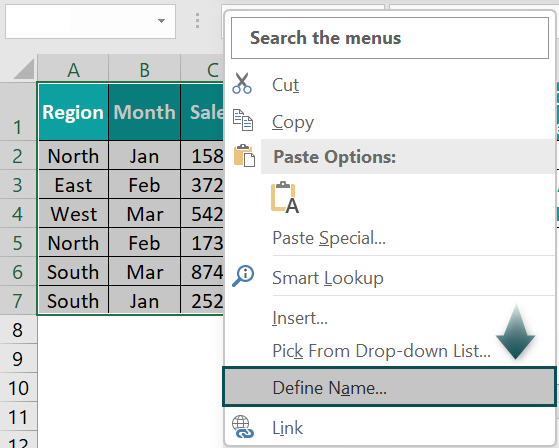
Example 3 - Address of the first cell in a range - Step 14

Step 15: A window called the New Name opens up.

Step 16: Set the table’s name; in this case, it is Data.

Step 17: Click OK.

Example 3 - Address of the first cell in a range - Step 17

Step 18: Then, select the column where we will enter the formula and calculate the result of the first cell address. The selected cell, in this case, is cell G2.

Step 19: Next, we will enter the Excel COLUMN, ROW, and ADDRESS formulas in cell G2.

Step 20: Enter the value of the row number argument as ROW(data), i.e., the range of rows.

Step 21: Similarly, enter the value of the column number argument as COLUMN(data), i.e., the range of columns.

Step 22: So, the complete formula entered is =ADDRESS(ROW(Data), COLUMN(Data)).

Example 3 - Address of the first cell in a range - Step 22

Step 23: Now, press Enter key. The result is obtained in cell G2 as $A$1.

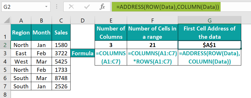
Example 3 - Address of the first cell in a range - Step 23

Likewise, we can use COLUMNS function in excel to get desired results.

Example #4 – Get The Address Of The Last Cell In A Range

The following example depicts the students’ marks, and we will calculate the address of the last cell in a range using the COLUMNS functions with the ROWS and ADDRESS functions in Excel.

In the table,

Column A, B, C, D, E, F, G, and H contains the roll number, name, marks, number of columns, number of cells in a range, first cell address of the data, and, last cell address of the data.
Row 3 contains the Formula.

COLUMNS Function in Excel - Example 4 - Address of the last cell in a range

The steps to calculate the number of columns, cells, and first cell addresses by the COLUMNS, ROWS & ADDRESS functions in Excel are as follows:

Step 1: First, select the column where we will enter the formula and calculate the result of the total number of columns. The selected cell, in this case, is cell E2.

Step 2: Next, we will enter the Excel COLUMNS Formula in cell E2.

Step 3: Then, enter the value of the array argument as A1:C7, i.e., the range of columns.

Step 4: Now, the complete formula entered is =COLUMNS(A1:C7).

Step 5: Next, press Enter key. The result is derived in cell E2 as shown in the image below.

Example 4 - Address of the last cell in a range - Step 5

Step 6: Then, select the column where we will enter the formula and calculate the result of the total number of cells. The selected cell, in this case, is cell F2.

Step 7: Next, we will enter the Excel COLUMNS Formula and ROWS formula in cell F2.

Step 8: Then, enter the value of the array argument as A1:C7, i.e., the range of columns.

Step 9: Similarly, enter the value of the array argument as A1:C7, i.e., the range of rows.

Step 10: Now, the complete formula entered is =COLUMNS(A1:C7) * ROWS(A1:C7).

Step 11: Press Enter key. The result is shown in cell F2 as 21.

Example 4 - Address of the last cell in a range - Step 11

Now, let us calculate the first cell address of the data.

Step 12: Select the table as A1:C7.

Step 13: Right-click on the selected table.

Step 14: Select the Define Name… option from the popped-up list.

Example 4 - Address of the last cell in a range - Step 14

Step 15: A window called New Name opens up.

Step 16: Set the table’s name; in this case, it is Data.

Step 17: Click OK.

Example 4 - Address of the last cell in a range - Step 17

Step 18: Select the column where we will enter the formula and calculate the result of the first cell address. The selected cell, in this case, is cell G2.

Step 19: Next, we will enter the Excel COLUMN, ROW, and ADDRESS formulas in cell G2.

Step 20: Enter the value of the row number argument as ROW(data), i.e., the range of rows.

Step 21: Similarly, enter the value of the column number argument as COLUMN(data), i.e., the range of columns.

Step 22: The complete formula entered is =ADDRESS(ROW(Data), COLUMN(Data)).

Step 23: Now, press Enter key. The result is obtained in cell G2 as shown in the image below.

COLUMNS Function in Excel - Example 4 - Address of the last cell in a range - Step 23

Next, let us calculate the last cell address of the data.

Step 24: Then, select the column where we will enter the formula and calculate the result of the last cell address. The selected cell, in this case, is cell H2.

Step 25: Next, we will enter the Excel COLUMN, ROW, and ADDRESS formulas in cell H2.

Step 26: Enter the value of the row number argument as ROW(data)+ROWS(data)-1, i.e., the range of rows.

Step 27: Next, enter the value of the column number argument as COLUMN(data)+COLUMNS(data)-1, i.e., the range of columns.

Step 28: So, the complete formula entered is =ADDRESS(ROW(Data)+ROWS(Data)-1,COLUMN(Data)+COLUMNS(Data)-1).

COLUMNS Function in Excel - Example 4 - Address of the last cell in a range - Step 28

Step 29: Now, press Enter key. The result is shown in cell H2 as $C$7.

COLUMNS Function in Excel - Example 4 - Address of the last cell in a range - Step 29

Important Things To Note

The COLUMNS Function in Excel accepts a single cell address or a range of cells as an argument.
The COLUMNS function cannot take multiple references as arguments.
If the array contains multiple rows and columns, only the columns are counted.
The COLUMNS function range reference must be a contiguous range.

Frequently Asked Questions (FAQs)

1. When to use Excel COLUMNS Function?

The Excel COLUMNS function is used when we want to count the number of columns in a specified range or array.

2. How does the COLUMNS function work in Excel?

The COLUMNS function works in Excel using the following steps;
• First, select an empty cell to enter the Formula.
• Next, type =COLUMNS( in the selected cell. Alternatively, type =C and double-click the COLUMNS function from the list of suggestions Excel shows.
• Then, press Enter key.

For example, the image below depicts the price of fruits, and we will calculate the total number of columns in a range using the COLUMNS functions in Excel.

The steps to calculate the number of columns by the COLUMNS Function in Excel are as follows:

• Step 1: First, select the column where we will enter the formula and then, calculate the result. The selected cell, in this case, is cell C2.

• Step 2: Next, we will enter the Excel COLUMNS Formula in cell C2.

• Step 3: Then, enter the value of the array argument as A1:B6, i.e., the range of columns.

• Step 4: So, the complete formula entered is =COLUMNS(A1:B6).

• Step 5: Now, press Enter key. The result is obtained in cell C2 as 2.

3. Where is the COLUMNS formula in Excel?

One can activate the COLUMNS Function in Excel using the following steps:
• First, choose the empty cell which will contain the result.
• Go to the Formulas tab and click it.
• Next, select the Lookup & Reference group.
• Then, select COLUMNS from the drop-down menu.
• A window called Function Arguments appears.
• As the number of arguments, enter the value in the array.
• Select OK.

Download Template

This article must help understand the COLUMNS Excel Function’s formula and examples. You can download the template here to use it instantly.

Columns in Excel Download

COLUMNS Function in Excel