LOOKUP in Google Sheets

What is LOOKUP Function in Google Sheets?

The LOOKUP function in Google Sheets looks for a specified value is a row or column and returns a corresponding value from the result range. LOOKUP is ideal for finding text and numeric data. It scans through the table or range given for a given key value and returns its corresponding value from the same position in another column/row of the range. Optimally, the search range should be sorted.

In the example below, we have some colors and their corresponding fruits. When you enter the following formula, you find that the search key “Green” has been detected by the function in the range A1:A6, and its corresponding value from B1:B6 is returned.

=LOOKUP(D3,A1:A6,B1:B6)

The LOOKUP function in Google Sheets is used to search a row or column for a value and return a corresponding value from another row or column.
The syntax of the LOOKUP function is as follows:

=LOOKUP(search_key, search_range, result_range)

a. search_key: The value we look for.

b. search_range: The range of cells to search for.

c. result_range: The range that contains the return value.

LOOKUP in Google Sheets can only search only one column or row at a time and can search both numeric and text values.
LOOKUP performs an approximate match by default if an exact match is not found.

Syntax

LOOKUP in Google Sheets allows users to easily search for particular data across rows and columns. Its syntax is simple and there are two ways of using it000.

=LOOKUP(search_key, search_range|search_result_array, [result_range])

search_key: The value you want to search for.
result_range (optional): The range from which the corresponding value will be returned once a match is found.

Approach 1 – Vector Mode

search_range: The range of cells where you want to search for the search_key. It is typically a single row or a column (one-dimensional).

Approach 2 – Array Mode

search_result_array -(optional): This range includes searches across multiple rows and columns. For horizontal arrays, it searches for the search_key in the first row000. For vertical arrays, it searches in the first column.

How to Use LOOKUP Function in Google Sheets?

The LOOKUP function in Google Sheets retrieves numeric values and text strings. It searches for a value in a range’s specified column/row and gives a result from a row/column. Let us look at how to enter the function in Google Sheets. There are two ways to do it.

Manually Enter LOOKUP
From the Google Menu Bar.

Manually Enter LOOKUP

Look at the data below. We have the IDs for some students and their names and ages. We must find the employee’s age with the ID as a lookup value.

Step 1: The first step is to write the LOOKUP function. We enter it in the following way.

=LOOKUP(3,A1:A7,C1:C7)

It follows the syntax of the VLOOKUP function in Google Sheets.

=LOOKUP(search_key, search_range, [result_range])

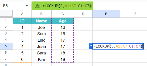
Step 2: Press Enter. You get the student age corresponding to the ID.

Using the Google Menu bar

We can also enter the same function using the Google Menu bar by going to “Insert” ➝ “Function” ➝ “Lookup” ➝ “LOOKUP.”
Enter the required arguments, close the bracket, and press the “Enter” key.

Examples

Google Sheets offers different types of LOOKUP functions, but the most common is LOOKUP. It is used to retrieve data based on a matching value. Let us look at a few interesting LOOKUP functions in Google Sheet examples featuring the same.

Example #1 – Using LOOKUP to Return a Text String

Let us look up the first example where we have a table with some flower name, pricing and description put up by a florist. Here, we have them sorted as well. Let us look up a flower’s description based on its name.

Step 1: Enter the details in the table.

Step 2: Now, to look up the description of lavender, enter the following function in an empty cell in Google Sheets.

=LOOKUP(“Lavender”, B2:B8, C2:C8)

“Lavender” is the search_key
B2:B8 is the search_range, the range where you search for the flower.
C2:C8 is the result_range from where the corresponding description is taken.

Step 3: Press Enter. The function searches for “Lavender” in the Flower column and returns the corresponding description from the Description column once it finds it.

Example #2 – Using LOOKUP to Retrieve Numeric Data

The advantage of the LOOKUP function is that it also retrieves text values. Let us use the same table above to retrieve a particular flower’s price.

Step 1: Enter the details shown below in a sheet.

Step 2: To find the price of the Lavender flower we used in Example 1, use the following function in an empty cell.

=LOOKUP(“Lavender”, A2:A8, B2:B8)

“Lavender” is the search_key
A2:A8 is the range where you search
B2:B8 is the range where the corresponding price is located.

Step 3: Press Enter. The function searches for “Lavender” in the Name column and returns the corresponding price from the Price(USD) column (C2:C5).

Step 4: What happens when the search value is not found? Do you get an N/A error like with VLOOKUP? If the search_key is not found, the search value used in the lookup will find the value immediately smaller in the range. For instance, here, we specify “Hyacinth” as the search value using the function.

=LOOKUP(“Hyacinth”, A2:A8, B2:B8). Press Enter.

You get the price of Daisy as D is the next smaller alphabet than H.

Example #3 – Using LOOKUP with VLOOKUP Function

The LOOKUP and VLOOKUP functions can be combined successfully for data retrieval. The VLOOKUP function searches for a value in the first column of a range and returns a result from a specified column to the right. We can perform more complex searches when it is combined with LOOKUP.

In this example, we want to find the price of a mobile phone using VLOOKUP. Here’s how we combine it with LOOKUP.

Step 1: Enter details in the table below.

Step 2: Enter the following function in an empty cell.

=VLOOKUP(LOOKUP(A10, A2:A7, A2:A7), A2:C7, 3, FALSE)

Here,

LOOKUP(A10, A2:A7, A2:A7) searches for OnePlus 11 in the range A2:A7. If it is present, it returns the same value as the key for the VLOOKUP.
=VLOOKUP(LOOKUP(A10, A2:A7, A2:A7), A2:C7, 3, FALSE) searches for the OnePlus 11 value in the table A2:C7. It returns the value from the 3rd column, the Price(USD) column.

Press Enter. You can see the price of the OnePlus 11 mobile phone being displayed using the combination of LOOKUP and VLOOKUP.

Important Things to Note

The LOOKUP function works properly only if the data in search_range or the search_result_array is sorted.
In case the data is not sorted, we may get different results. In this case, we can go for the VLOOKUP or HLOOKUP functions.
If the data in the column or row is not sorted, you can also use the SORT function for sorting.
You must specify the single column or row to return for the result.
If the search_key is not found, you do not get an error. Instead, the search value used in the lookup will find the value immediately smaller in the range.
If you use the search_result_array (vector) method, the last row or column in the provided range is returned.

Frequently Asked Questions (FAQs)

What is the difference between LOOKUP, HLOOKUP, and VLOOKUP in Google Sheets?

LOOKUP: Searches for a value in a row or column and can return values from another row or column. It works only when the data is sorted in ascending order. To find an exact match, type the name accurately in the search key argument.

VLOOKUP: Looks for a value in the first column of a range (vertical lookup) and returns the corresponding value from another column. It searches vertically for a value in a row and returns data left-to-right. Here, data doesn’t have to be sorted. Using the fourth argument as FALSE, you can find exact matches.

What ere the Limitations of LOOKUP in Google Sheets?

1. The biggest issue with LOOKUP is that it can return incorrect results without any error messages or warnings. If there are multiple entries like duplicates, it may return any one value which may not be the one you need.
2. For LOOKUP to work accurately, we require the data to be sorted in ascending order.
3. Functions like HLOOKUP and VLOOKUP have better performance and allow to specify different types of matches without the need to sort the data.

What are the common errors when you use the LOOKUP in Google Sheets?

The common errors you may encounter in Google Sheets include:

• #VALUE!: It occurs if the data in search_range is not sorted in ascending order for matches.
• #REF!: If the result_range is smaller than search_range, you may get a reference error.

Download Template

This article must help understand LOOKUP Function in Google Sheets with its formulas and examples. You can download the template here to use it instantly.

LOOKUP Function In Google Sheets Download

LOOKUP in Google Sheets