Pivot Table Field Name Is Not Valid

What Is Pivot Table Field Name Is Not Valid Error?

The Pivot Table field name is not valid error occurs when one creates a Pivot Table based on a dataset with one or more columns without the headers or empty columns. Also, the error can occur when we delete one or more column headers, columns or the entire source dataset and refresh the inserted Pivot Table.

Users can avoid this error bacy ensuring all the required columns in the source dataset have headers, and the columns are not empty. On the other hand, they can avoid the error by not selecting the entire sheet while creating a Pivot Table.

For example, the following image shows a list of employees, their departments and three days of salaries.

Inserting a Excel Pivot Table based on the abovementioned source data is the requirement.

Then, we can use the PivoTable option in the Insert tab to create the required Pivot Table.

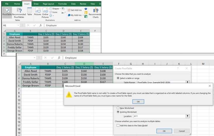
So, we select the source dataset and choose the PivotTable option in the Insert tab to open the Create PivotTable window. It shows the chosen data range in the Table/Range field.

We update the target cell address in the Location field under the Existing Worksheet option in the Create PivotTable window to display the required Pivot Table in the current sheet.

Next, when we click OK in the Create PivotTable window, we see the Pivot Table field name is not valid error message.

The reason for the error is that column B is missing the header. Hence, for the error Pivot Table field name is not valid labeled columns are the solution.

So, once we update the column B label, say, as Department, we will not see the error message, and we can successfully create the required Pivot Table for the source data.

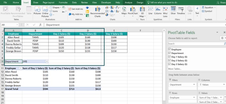
Thus, while the VBA Pivot Table field name is not valid error is possible; the above example shows that the error can occur when creating a Pivot Table without VBA coding.

How To Solve This Error?

The following scenarios explain the Pivot Table field name is not valid meaning, and we shall see the solution to overcome the error in each case.

#1 – Without Header Value, We Cannot Create A Pivot Table

When we try creating a Pivot Table based on a dataset containing columns without headers, we cannot create it. Instead, we will see the Pivot Table field name is not valid error.

Thus, here is how to use the Pivot Table field name is not valid labeled columns as the solution.

1. Select the first cell of the column which is missing the header in the source dataset. Next, enter the appropriate heading in the chosen cell. Likewise, update the headers for all the columns with missing headers in the source dataset.
2. Select the source dataset and choose the Insert tab – PivotTable option to open the Create PivotTable window.
3. Ensure the chosen source data range is correct and update the target location in the Create PivotTable window where we wish to place the Pivot Table. It could be a new sheet or a cell in the existing sheet.
4. Click OK in the Create PivotTable window.

Finally, Excel will show the target location and the PivotTable Fields pane. We can drag and drop the concerned fields in the required areas in the PivotTable Fields pane to achieve the desired Pivot Table at the chosen location in the Excel file.

Basic Example

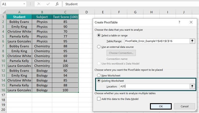
The following source dataset lists students and their test scores in different subjects.

The aim is to create a Pivot Table based on the source data.

Step 1: Choose the source data range A1:C16 and select Insert – PivotTable.

The Create PivotTable window opens, showing the source dataset range in the Table/Range field required to analyze.

However, the specified range excludes the column C cells since the last column header in the source dataset is blank.

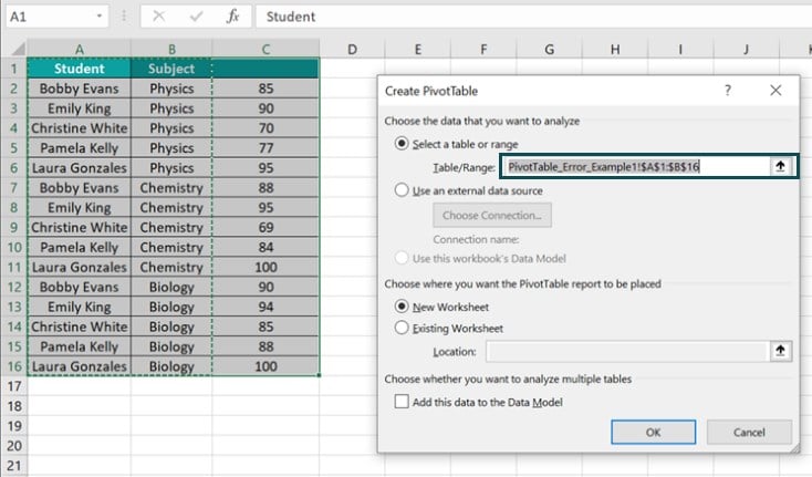
So, click inside the Table/Range field and update the correct source data range.

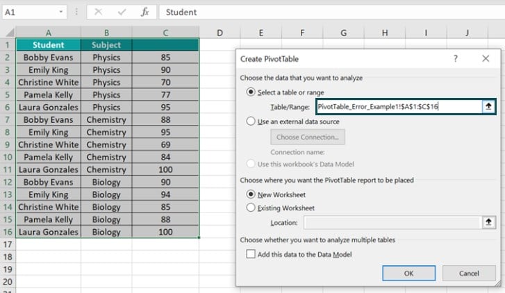
Step 2: We shall show the Pivot Table in the current sheet. So, select the Existing Worksheet option and update the target cell address in the Location field.

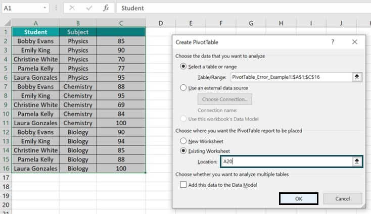
However, clicking OK in the Create PivotTable window will show the following error message.

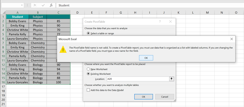
Step 3: Click OK to close the warning message box showing the error and close the Create PivotTable window.

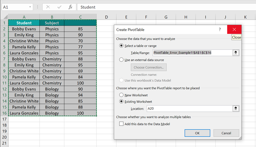
Step 4: Choose cell C1 and update the appropriate column heading.

Step 5: Select the source data range A1:C16 and choose the Insert tab – PivotTable option.

The Create PivotTable window opens, showing the correct source data range in the Table/Range field.

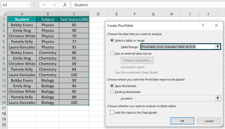
Step 6: Choose the required target location in the Create PivotTable window, where we aim to place the Pivot Table.

Next, click OK in the Create PivotTable window.

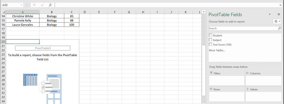
Excel will no longer show the error. Instead, we will see the target location in the sheet, where we can place the required Pivot Table and the PivotTable Fields pane to create the Pivot Table.

Step 7: Drag and drop the required fields in the specific areas in the PivotTable Fields window to insert the required Pivot Table in the chosen target location in the sheet.

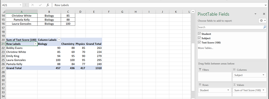
Step 8: Select cells A21 and B20 individually to update the row and column labels according to our requirements.

Thus, the final Pivot Table will be as shown below:

#2 – Column Header Deleted After Creating A Pivot Table

Sometimes, we will create the Pivot Table based on the source dataset. But, when we delete one or more column headers, we get the error Pivot Table field name is not valid when refreshing the inserted Pivot Table.

Thus, the following steps will help overcome the error in such a scenario.

1. Select the first cell of the column in the source dataset without the header. And update the required label in the chosen cell. Likewise, update the headers of all the columns which are missing the headers.
2. Right-click a cell in the Pivot Table and select Refresh from the contextual menu.

So now, we will not get the error Pivot Table field name is not valid when refreshing the inserted Pivot Table.

Basic Example

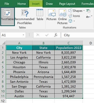
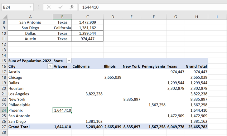
The following source dataset lists US cities and their states and population statistics for 2022.

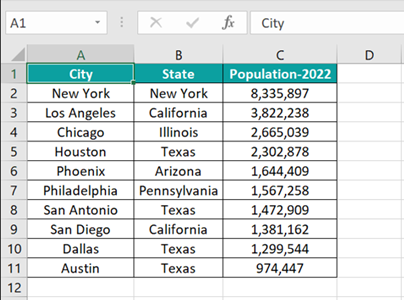
The requirement is to insert a Pivot Table for the given dataset.

Step 1: Choose the cell range A1:C11 and select Insert – PivotTable to access the Create PivotTable window.

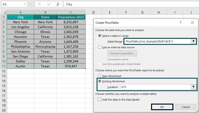
Step 2: Since the source dataset is complete, the Table/Range field in the Create PivotTable window will show the correct data range.

Next, update the target location in the window, where we aim to place the Pivot Table and click OK.

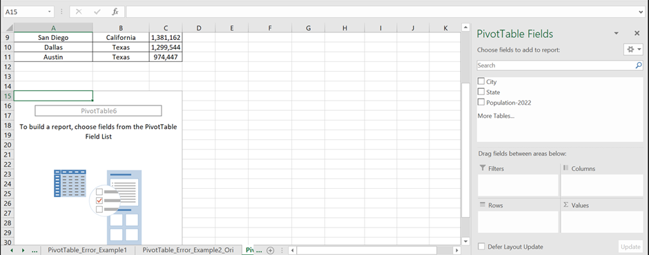
While we can see the target location in the sheet to place the required Pivot Table, the PivotTable Fields pane will open.

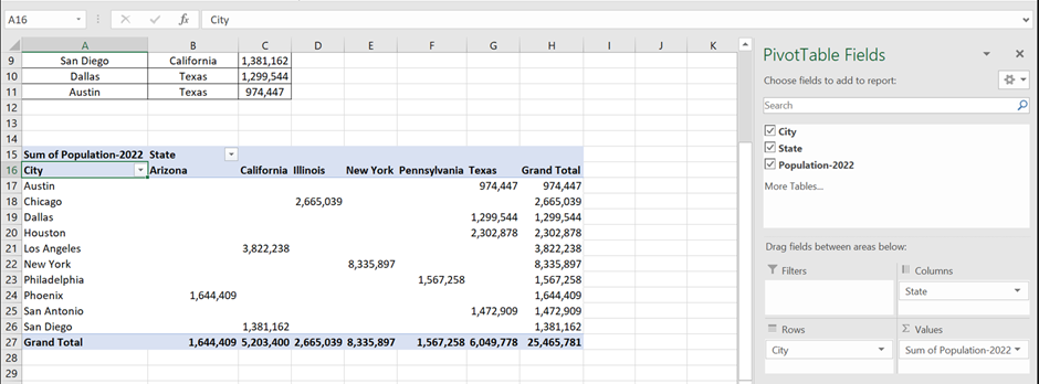
Step 3: Drag and drop the concerned fields in the appropriate areas in the PivotTable Fields window to achieve the required Pivot Table in the target cell.

Next, assume we delete the column C header.

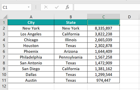
After that, choose cell C6 to update Phoenix’s population.

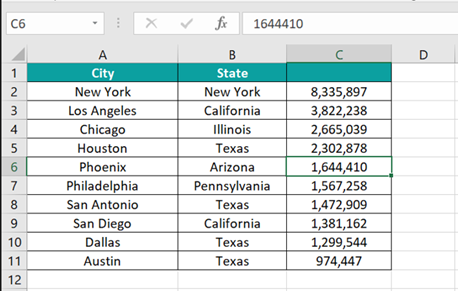
Step 4: Right-click a cell in the Pivot Table and choose Refresh from the context menu to view Phoenix’s updated population figure in the Pivot Table.

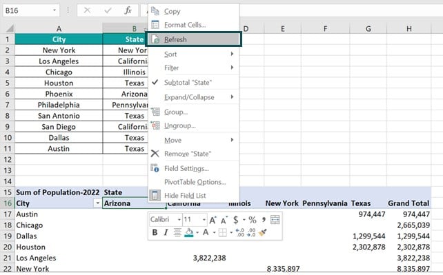
However, the error message will appear, as depicted in the below image. Click OK to close it.

Step 5: Thus, we choose cell C1 in the source dataset and update the column header as a solution.

Next, right-click a cell in the Pivot Table to choose Refresh in the context menu.

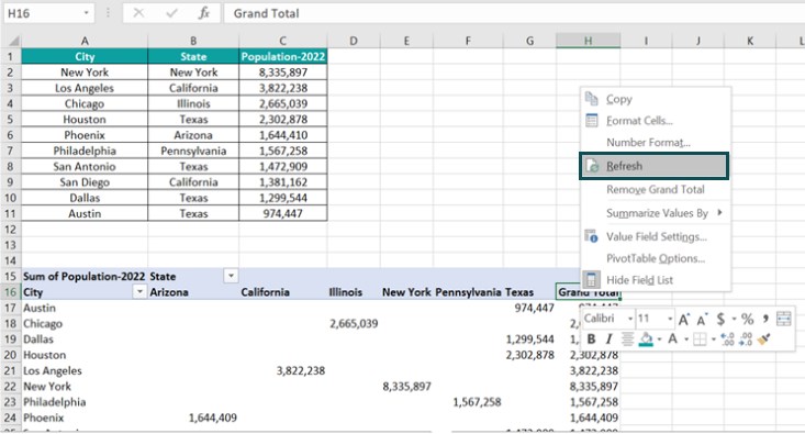
We will no longer get the error. Instead, we will see the updated population figure for Phoenix in the Pivot Table.

#3 – Entire Data Deleted After Creating A Pivot Table

Consider we create a Pivot Table based on the source dataset. But for some reason, we must delete the entire source dataset.

In such a scenario, when we refresh the Pivot Table, Excel will show the invalid Pivot Table field name error.

Thus, we should avoid deleting the entire dataset after building a Pivot Table based on it.

Basic Example

The following image shows a source dataset containing a firm’s branch offices and their zones and sales data.

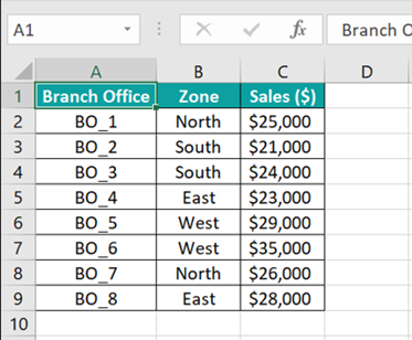
We select the source data range and use the Insert – PivotTable option to create the required Pivot Table.

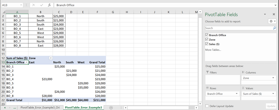
Next, let us see what happens when we delete the source dataset.

Step 1: Choose the source dataset range A1:C9.

Next, press Delete to delete the entire dataset.

Step 2: Right-click a cell in the Pivot Table to choose Refresh from the contextual menu.

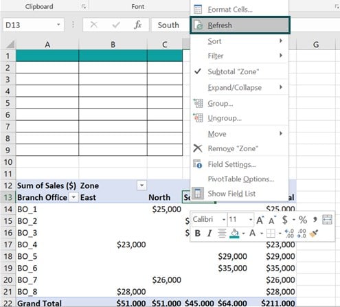
Excel will show the invalid Pivot Table field name error. Click OK to close it.

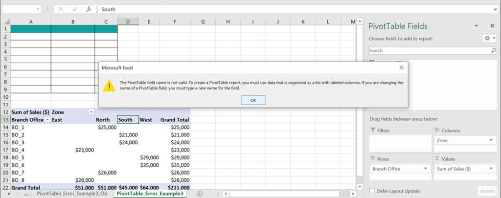
Thus, it is best to avoid deleting the entire source dataset after inserting the Pivot Table.

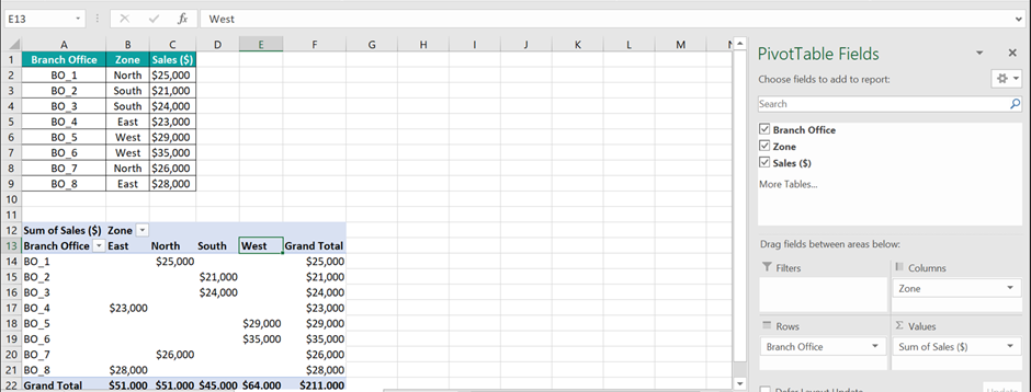
So, restore the source dataset in the same range and right-click a cell in the Pivot Table to select the Refresh option in the contextual menu. Then, the Pivot Table will get refreshed without any error.

#4 – Selecting The Entire Sheet And Try Creating A Pivot Table

Sometimes, we may select the entire worksheet to create the Pivot Table, even with a source dataset in a specific cell range.

Excel will not let us insert the required Pivot Table in such a scenario. Instead, it will show the invalid Pivot Table field name error.

Thus, the only solution is to avoid selecting the entire sheet and only choose the required source data range to create the desired Pivot Table.

Basic Example

The following image shows a source dataset containing a set of fruits and their grades and units ordered data.

The aim is to create a Pivot Table based on the source dataset.

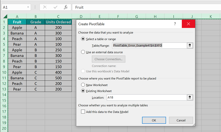
Step 1: Click the Green triangle on the top-left corner of the workspace to select the entire sheet.

Next, select Insert – PivotTable to access the Create PivotTable window.

Step 2: Since the source dataset is in columns A:C, the range is displayed accordingly in the Table/Range field in the Create PivotTable window.

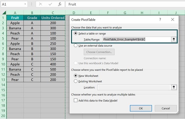
So, we shall update the data range in the Table/Range field to ensure the entire sheet is selected while creating the Pivot Table, as depicted in the image below.

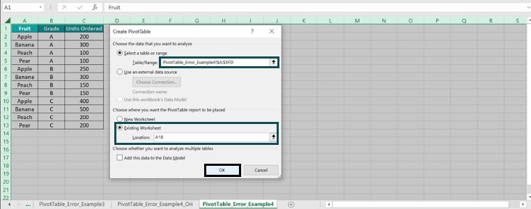
Next, update the target location, where we aim to place the Pivot Table and click OK in the Create PivotTable window.

We will see the invalid Pivot Table field name error message.

Click OK to exit from the error message box and close the Create PivotTable window.

Step 3: Select the source dataset range A1:C13 and choose the PivotTable option in the Insert tab.

The Create PivotTable window opens, showing the correct source data range in the Table/Range field.

Next, we can update the target location in the Create PivotTable window, where we plan to place the required Pivot Table and click OK.

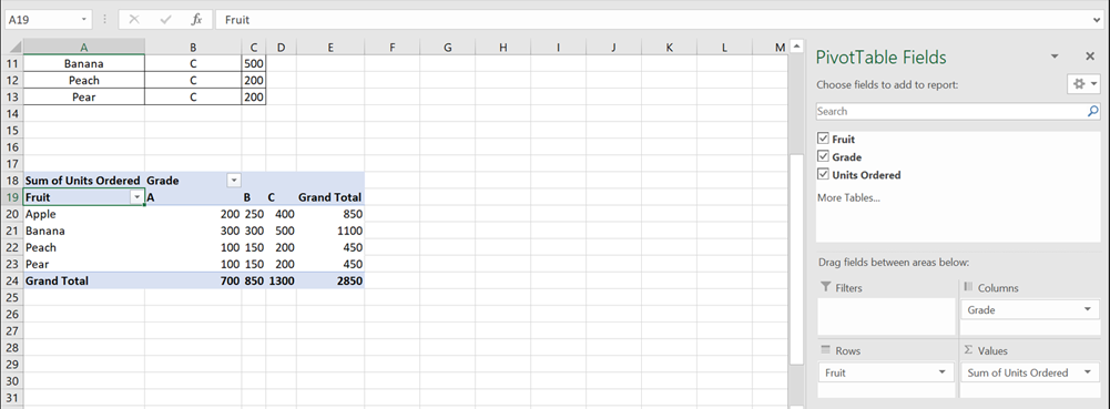
Excel will no longer show the error message. Instead, we can view the space to insert the Pivot Table in the target location and the PivotTable Fields pane to create the desired Pivot Table, shown below.

#5 – Blank Column In The Data

When we try creating a Pivot Table based on a dataset containing one or more blank columns, we may see an error similar to the VBA Pivot Table field name is not valid.

Thus, here is how to avoid the invalid Pivot Table field name error in such cases.

1. Ensure the data range chosen to create a Pivot Table does not contain blank columns.
2. Use Steps 2 to 4, explained in section #1 – Without Header Value, We Cannot Create a Pivot Table to insert the required Pivot Table at the desired location in Excel.

Basic Example

The image below shows a dataset listing the sales representatives at a firm, their teams and the monthly sales they generated.

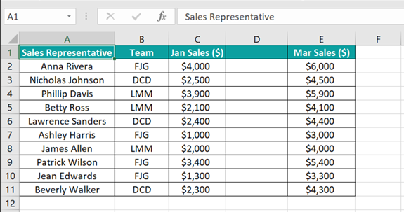
The aim is to insert a Pivot Table based on the above dataset.

Step 1: Choose the dataset range A1:E11 and select the Insert – PivotTable option.

Step 2: The Create PivotTable window opens, where the Table/Range field shows the chosen data range.

Update the location in the Create PivotTable window, where we aim to insert the Pivot Table in Excel.

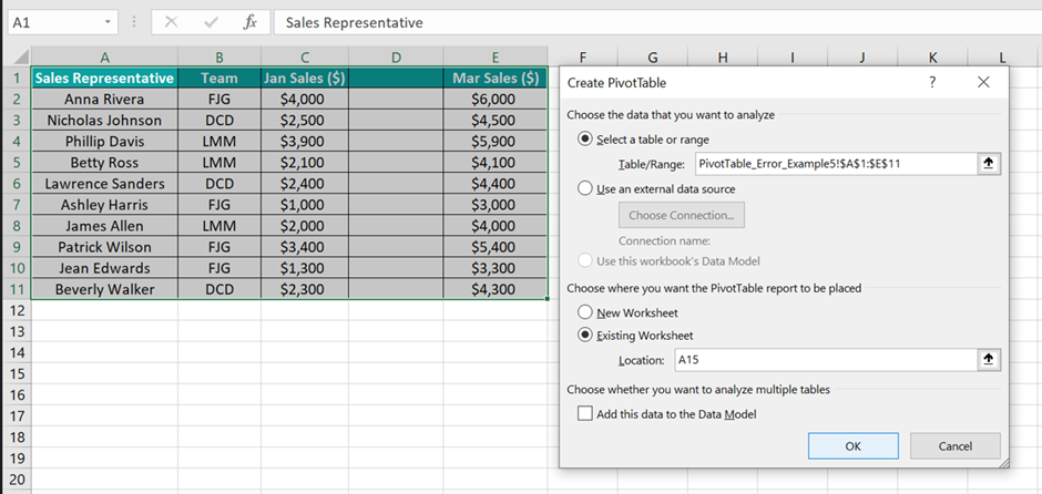
However, clicking OK will result in the invalid Pivot Table field name error since column D in the source dataset is empty.

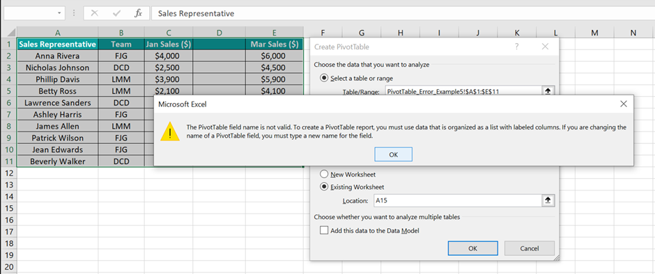
Click OK to exit the warning message box and close the Create PivotTable window.

Step 3: Update the required data in the column D cells, including the column header. Otherwise, if we do not need column D, click the column D heading to select the column and right-click to choose Delete from the contextual menu to remove the empty column.

Next, choose the entire dataset A1:E11 and the Insert tab – PivotTable option.

The Create PivotTable window opens, with the Table/Range field showing the chosen source dataset range.

Next, update the location in the Create PivotTable window, where we want to insert the required Pivot Table.

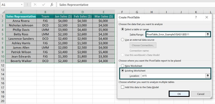
Clicking OK in the Create PivotTable window will not show the error message. Instead, we will see the specified target location and the PivotTable Fields window required to insert the Pivot Table.

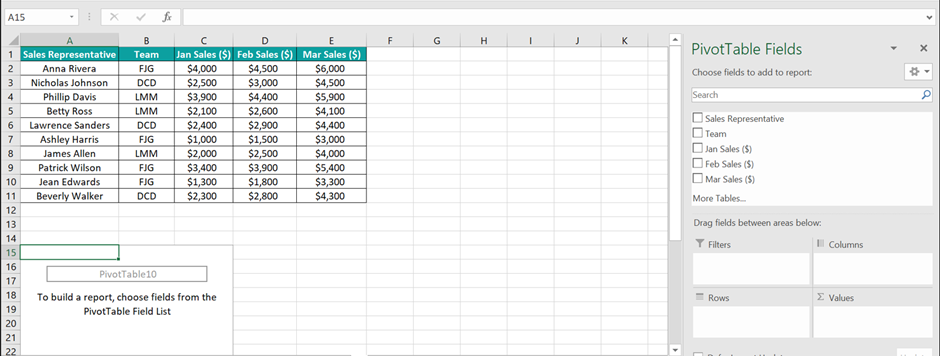
Finally, dragging and dropping the required fields in the concerned areas in the PivotTable Fields pane will result in the required Pivot Table, shown below:

Thus, the above-explained scenarios with practical examples help us understand the Pivot Table field name is not valid meaning effectively.

Important Things To Note

• Consider the last column in the source dataset does not have a header. Then, the Table/Range field in the Create PivotTable window will show the data range from the first column to the second-last column in the source dataset. So, we must manually update the data range to include the last column in the Table/Range field. But still, Excel will show the Pivot Table Field Name Is Not Valid error due to the missing column header.
• The invalid Pivot Table field name error can occur before or after developing a Pivot Table based on the source dataset.

Frequently Asked Questions (FAQs)

Download Template

This article must be helpful to understand the Pivot Table Field Name Is Not Valid, with its formula and examples. You can download the template here to use it instantly.

Recommended Articles

This has been a guide to What Is Pivot Table Field Name Is Not Valid. We learn to solve/fix the error in different scenarios, with examples & points to remember. You can learn more from the following articles –

• Pivot Table Change Data Source
• Power BI Pivot Table
• Pivot Table Slicer