What Is Protecting Excel Sheet?
Protect Sheet in Excel is an option that enables us to lock the required cells in a worksheet and password-protect the sheet. It ensures other users can edit, move, or delete data from only certain parts of the protected sheet, with other parts being unmodifiable.
Users can utilize the Protect Sheet option to protect cell ranges, shapes, charts, and ActiveX controls and hide formulas from unnecessary changes in a sheet.
📥Download the ready-to-use Excel template to practice this tutorial yourself.
Protect-Sheet-in-ExcelFor example, the following image shows a worksheet containing students and their ranks.
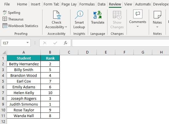
And the task is to confirm that other users do not modify the sheet content.
Then, using the Protect Sheet option to password protect sheet in Excel can help us meet our requirements.
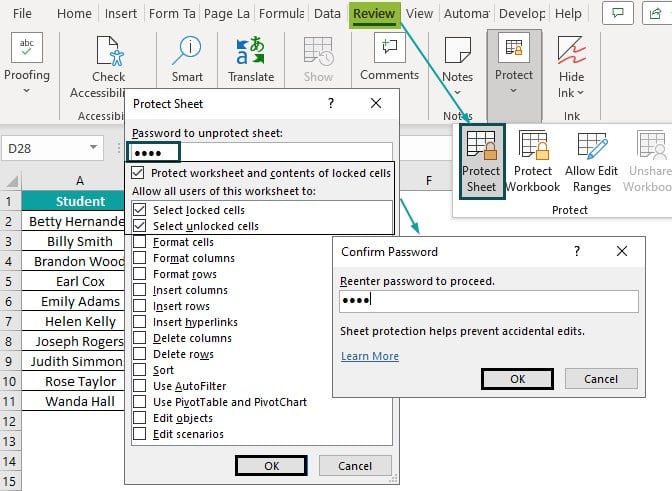
In the above password protect sheet in Excel example, we choose the Protect Sheet option in the Review tab to access the Protect Sheet window. And then, we update the password in the Protect Sheet window and select the actions other users can perform in the protected sheet.
Next, once we click OK, Excel will open the Confirm Password window to reconfirm the password. Finally, clicking OK in the Confirm Password window will protect the current worksheet.
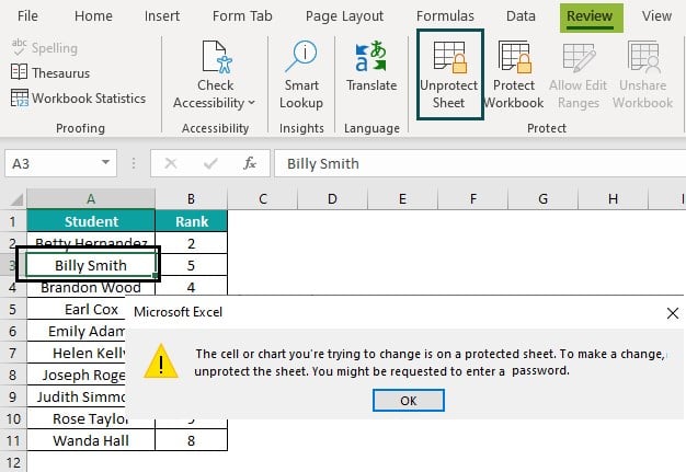
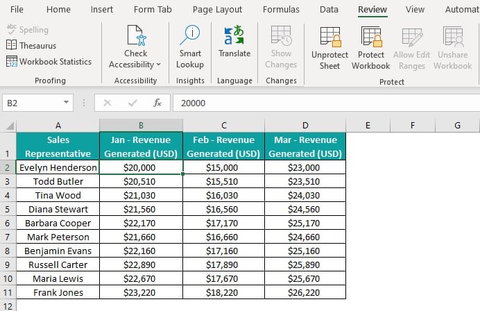
And the Protect Sheet command in the Review tab changing to Unprotect Sheet confirms the same.
So now, if a user tries editing a cell in the sheet, say, cell A3, Excel will show a warning message stating the cell is in a protected sheet. And they must unprotect the sheet to make changes in the sheet.
Thus, the data in the sheet is protected from unauthorized users.
Table of contents
Key Takeaways
- Protect Sheet in Excel is a feature for locking a cell, range, formulas and password-protect a worksheet. It ensures unauthorized users cannot edit data in specific parts of a protected sheet.
- Users can use Protect Sheet in Excel to protect sheet elements such as data, Sparklines and SmartArt and prevent other users from modifying the elements.
- We can utilize the Protect Sheet option from the Review tab or the context menu to access the Protect Sheet window for protecting a worksheet.
- We can access the Format Cells window to lock cells and lock and hide formulas in a worksheet, after which we must protect the sheet to complete the action.
How To Protect A Sheet In Excel?
The steps to protect sheet in Excel are as follows:
- Open the worksheet we wish to protect and choose the Review tab – Protect Sheet option.

[Alternatively, right-click the sheet tab we wish to protect, and choose Protect Sheet in the contextual menu.

Otherwise, use the keyboard shortcut to Protect Sheet in Excel, Alt + T + P + P.]
The above step will open the Protect Sheet window.

2. Type the password in the first field in the Protect Sheet window.
Next, the window shows a list of actions we can allow the users to perform in the protected sheet. So, let us select the first two options.

Clicking OK in the Protect Sheet window will open the Confirm Password window.

3. Next, reenter the password we entered in the Protect Sheet window in the Confirm Password window.

4. Click OK in the Confirm Password window to achieve the protected worksheet.

Please note that the password update in the Protect Sheet window is optional. If we skip it and click OK in the Protect Sheet window, the Confirm Password window will not appear. And the sheet will appear protected.
However, the drawback is that unauthorized users can click the Unprotect Sheet option in the Review tab and unprotect the sheet without a password.
Basic Example
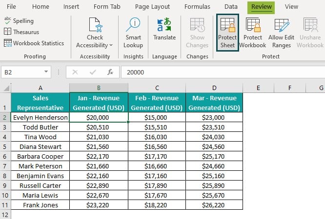
The following image shows a worksheet.

And here is the method to protect it.
Step 1: Select Review – Protect Sheet or use the keyboard shortcut to Protect Sheet in Excel, Alt + T + P + P, which will open the Protect Sheet window.
Step 2: Enter the password and choose the actions a user can perform in the protected sheet in the Protect Sheet window. And then click OK.
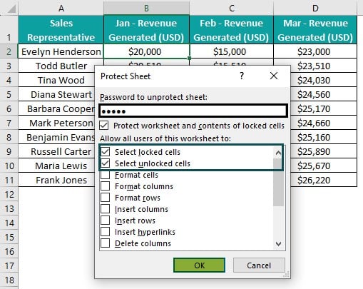
Step 3: The Confirm Password window opens, where we must enter the password we updated in the Protect Sheet window.

Step 4: Click OK in the Confirm Password window to reconfirm the password and obtain the protected sheet.
How To Protect Cells In An Excel Worksheet?
The primary use of Protect Sheet in Excel is that the feature enables us to lock specific cells while leaving the remaining cells editable for the users.
And the method to protect cells in a worksheet is as follows:
- Click on the triangle at the top-left corner above the sheet’s work area to select all the cells.
- Right-click to open the contextual menu and click on the Excel Format Cells option. Otherwise, press Ctrl + 1.
- The Format Cells window will open, where we should click the Protection tab to open it.
- Check the Locked option in the Protection tab and click OK. This step ensures that all the cells in the sheet are locked.
- Choose the cells which must be editable. Next, right-click to access the contextual menuand click on Format Cells.
- Click the Protection tab in the Format Cells window to open the tab.
- Uncheck the Locked option in the Protection tab. And then click OK to unlock the chosen cells in the sheet.
- Select Review à Protect Sheet to access the Protect Sheet window.
- Type the password in the Protect Sheet, which is optional.
- Click OK in the Protect Sheet window to protect the sheet with all the cells locked except those chosen.
Basic Example
The following example explains the main use of Protect Sheet in Excel, locking specific cells in a worksheet.
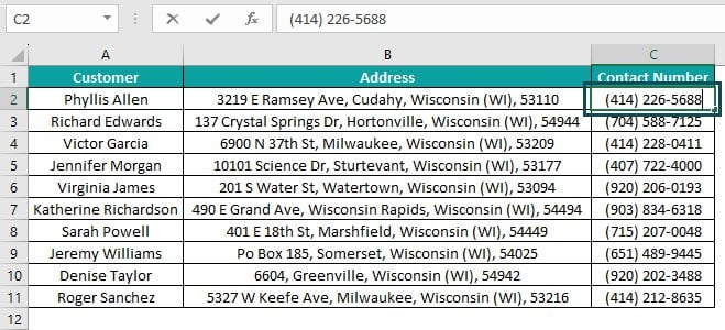
The following image shows a worksheet containing customer details.
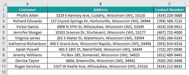
The requirement is to protect all the cells in the sheet, except those containing customer details (cells A2:C11), so that the specified cells are editable.
Then, the steps are as follows:
Step 1: Click on the triangle in the top-left corner above the work area to select all the cells in the sheet.
Next, right-click to open the context menu and choose Format Cells to access the Format Cells window.

Step 2: Click the Protection tab in the Format Cells window to open it. And check the Locked option.

And click OK.
Step 3: Click on cell A2. And then, while holding the mouse’s left key, drag the mouse over columns B and C cells to choose the range A2:C11.
Next, right-click to access the contextual menu and click on Format Cells.
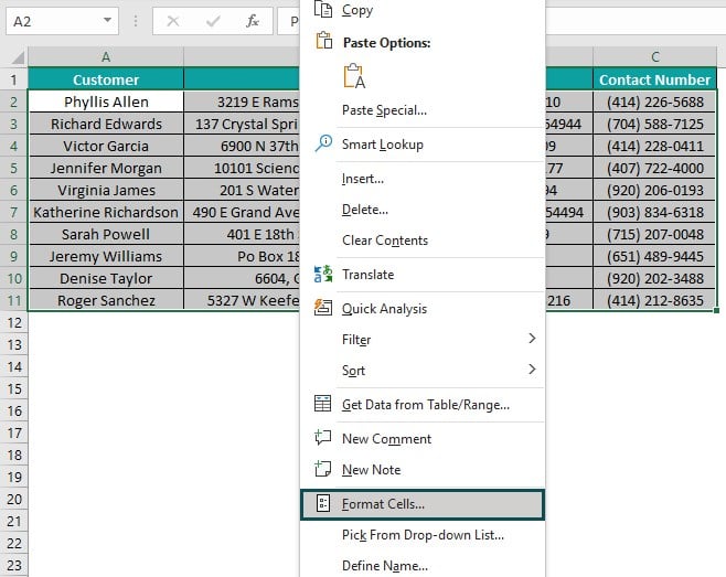
Step 4: The Format Cells window will open, where we should click the Protection tab to open it and uncheck the Locked option.
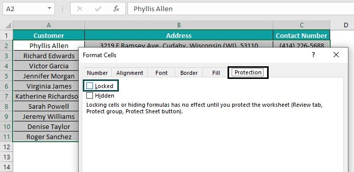
And click OK.
Step 5: Choose Review – Protect Sheet.
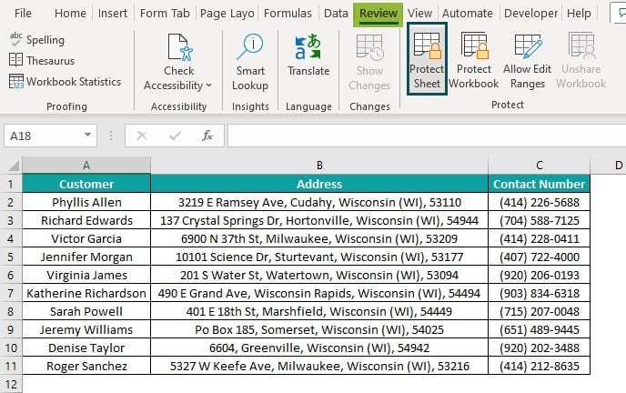
Step 6: The Protect Sheet window opens, where will select the first two actions the users can perform in the protected sheet.
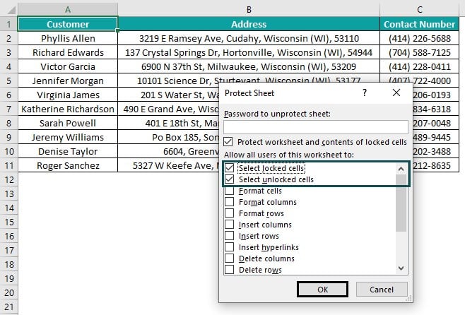
Finally, clicking OK in the Protect Sheet will protect the sheet, with all the cells locked, except A2:C11.
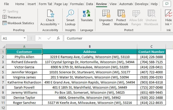
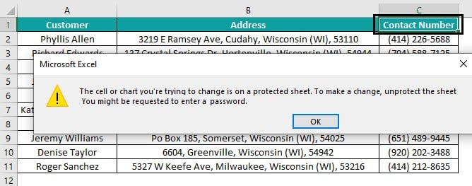
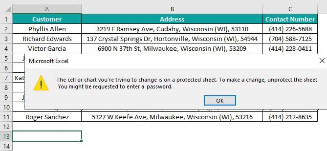
Furthermore, we can confirm by double-clicking the locked cells, such as C1 and A13. In both cases, Excel will show the protected sheet warning message.
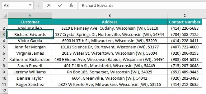
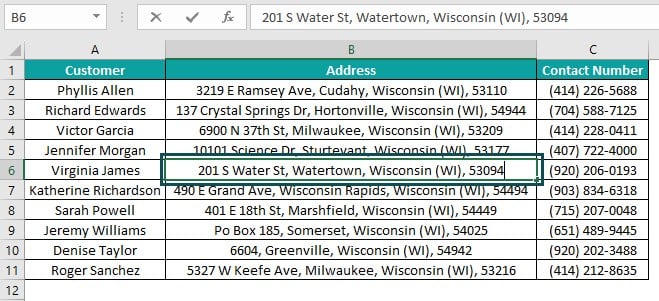
But double-clicking the unlocked cells, such as A3, B6, and C2, shows the cells are editable.
How To Hide The Formula Associated With A Cell?
The steps to hide a formula associated with a cell using the Protect Sheet in Excel from view option are as follows:
- Click on the triangle at the top-left corner above the work area to select all the cells in the sheet. Next, right-click to access the context menuand click on Format Cells.
- Open the Protection tab and select the Locked option in the Format Cells window. And click OK.
- Choose the cell or range containing the formula or formulas we aim to hide.
- Right-click the chosen cell or range and select Format Cells in the contextual menu.
- Open the Protection tab and select the Locked and Hidden options in the Format Cells window. And click OK.
- Select Review à Protect Sheet to access the Protect Sheet window.
- Enter the password (optional) and choose the actions the users can perform in the protected sheet in the Protect Sheet window. And then click OK.
Thus, the sheet becomes protected, and the formulas in the chosen cell or range will not be visible in the Formula Bar or the cell or range.
Basic Example
The following dataset shows arithmetic operations, with cells E2:E5 containing formulas.
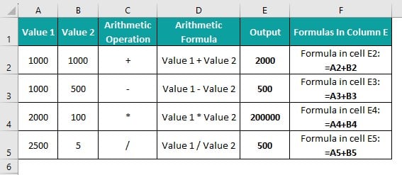
So, here is how to hide the formulas using the Protect Sheet in Excel from view option.
Step 1: Click on the triangle at the top-left corner above the workspace to select all the cells in the sheet.
Next, right-click to access the context menu and click on Format Cells.

Step 2: The Format Cells window will open, where we should click the Protection tab to open it and check the Locked option. And then click OK.
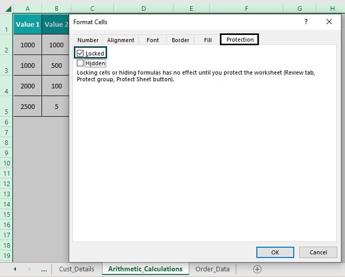
Step 3: Choose the range E2:E5. Next, right-click to access the contextual menu and click on Format Cells.
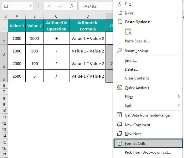
Step 4: The Format Cells window will open, where we should choose the Protection tab.
And then, select the Locked and Hidden options and click OK.
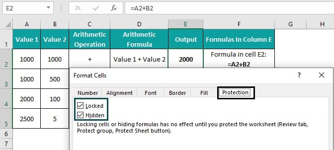
Step 5: Choose Review – Protect Sheet to access the Protect Sheet window.
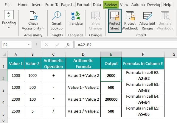
And choose the actions the users can perform in the protected sheet in the Protect Sheet window.
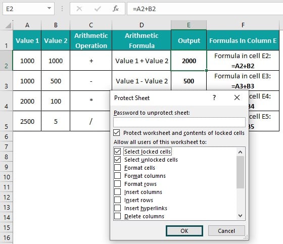
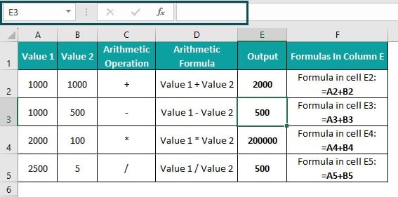
Finally, click OK to view the protected sheet.
And now, when we select cells in the range E2:E5, the formulas will remain hidden or protected from viewing and editing. And they will not show in the Formula Bar.



Pros & Cons
The pros and cons of the option Protect Sheet in Excel are as follows:
Pros
- It prevents users from editing or modifying data in a worksheet accidentally.
- It prevents unauthorized users from deliberately making changes to a worksheet.
- It enables us to ensure the users can perform only the permitted actions in the protected sheet specified in the Protect Sheet window.
Cons
- It is not a security feature. And hence, it does not lock the workbook structure.
- It does not protect the remaining sheets in the Excel file from users moving, editing, adding, deleting, and hiding them.
Important Things To Note
- The password we use to protect sheet in Excelis case-sensitive and not recoverable.
- Consider we protect a sheet without checking any actions that users can perform in the protected sheet. Then, users can only view the protected sheet.
- We must protect the worksheet after locking and hiding cells. Otherwise, the cells will not get locked or hidden for protection.

Frequently Asked Questions (FAQs)
You can password protect a sheet in Excel from viewing.
For example, the following image shows a workbook, with the Order_Data tab being the current sheet.
Consider we must password-protect the Order_Data sheet from viewing. Then, the steps are as follows:
Step 1: Right-click the Order_Data tab and choose Hide in the context menu to hide the sheet.
Step 2: Select Review – Protect Workbook to open the Protect Structure and Workbooks window.
Step 3: Enter the password and ensure the Structure option is checked in the Protect Structure and Workbooks window.
Clicking OK in the Protect Structure and Workbooks window will open the Confirm Password window to reenter the password for confirmation.
And clicking OK in the Confirm Password window will password-protect the workbook.
So now, when we right-click a visible sheet tab in the protected workbook, the Unhide option appears greyed out in the context menu. And hence, we cannot unhide and view the Order_Data sheet we hid.
The Protect Sheet is greyed out in Excel, perhaps because of the following reasons:
• The worksheet is in a shared workbook.
Solution:
1. Select Review – Share Workbook to open the Share Workbook window.
2. Uncheck the option to use the old shared workbooks feature rather than the new co-authoring experience in the Editing tab in the Share Workbook window.
3. Click OK in the Share Workbook window to unshare the workbook and view the Protect Sheet option enabled in the Review tab.
• We selected multiple sheets in the workbook.
Solution:
1. Right-click on one of the chosen sheets and select Ungroup Sheets in the context menu to unselect the chosen sheets and enable the Protect Sheet option.
2. Click on one of the unchosen sheet tabs to deselect all the sheets in the workbook and enable the Protect Sheet option.
Protect sheet vs. workbook in Excel is that Protect Sheet enables us to lock cells and helps prevent data modification and formatting.
But Protect Workbook lets us prevent worksheet addition, deletion, hiding, unhiding, and moving.
Download Template
📥Download the ready-to-use Excel template to practice this tutorial yourself.
Protect-Sheet-in-ExcelRecommended Articles
This has been a guide to What Is Protect Sheet In Excel. We learn how to protect sheet, cells, & hide the formula in a cell with examples and pros & cons. You can learn more from the following articles –

Leave a Reply