RANK Function In Google Sheets

What Is RANK Function In Google Sheets?

RANK function in Google sheets, as the name suggests, helps users find the rank, also known as position of a value in the data. It is a default function and finds the rank in ascending order or descending order. There are three functions available under RANK function category. They are RANK function with arrays, RANK.EQ and RANK.AVG Google sheets function.

For example, consider the below table showing names and marks in columns A and B, respectively.

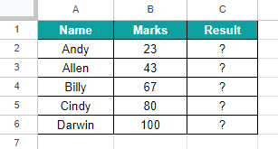
Now, let us learn how to find the rank of values in the data using RANK function.

To begin with, select the cell C2 and insert the Google sheets RANK function formula =RANK(B2,$B$2:$B$6) and press Enter key. We will be able to find the rank or position of the value in cell B2. Now, using AutoFill option, we can find the result in the cell range C3:C6, as shown in the below image.

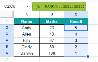
Likewise, we will be able to find the rank or position in Google sheets.

In this article, let us learn how to use the Google sheets RANK function with detailed examples.

RANK() Google Sheets Formula

The formula or syntax of RANK function is =RANK(value,data,[is_ascending])

where

• Value is the value or numeric data to be ranked or positioned
• Data is the array or cell range in the data used for ranking

Both the arguments are mandatory.

• Is_ascending is the only optional argument used to show if the ranking is in the ascending or descending order.
• For assigning the rank or position in ascending order, we need to use 1 or TRUE
• Likewise, to rank the data in descending order, we need to use 0 or FALSE

How To Use RANK Function In Google Sheets?

We can insert the RANK function in two ways. They are:

• Include the formula from Insert tab
• Manually enter the formula in Google sheets

Let us learn how to insert the RANK function in Google spreadsheets with the help of following steps.

Method #1 – Include the Formula From Insert Tab

Step 1: First, select the cell where we want to find the result.

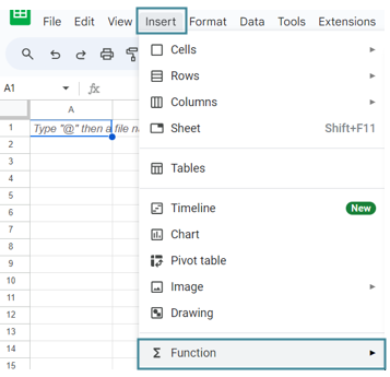
Step 2: Next, click on the Insert tab. Click on Function.

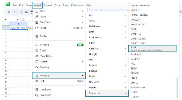
Step 3: In the options, click on Statistical. Select RANK function to insert the RANK function in the cell.

Method #2 – Manually Enter the Formula in Google Sheets

Step 1: To begin with, select the cell where we want to find the result.

Step 2: Type =RANK or alternatively, type =R. Then select the formula in the list of options that appear.

Step 3: Enter the arguments. Press Enter key.

We will be able to find the result using RANK function in Google sheets.

Likewise, we can use RANK function in Google sheets.

Examples

Let us learn how to use RANK function with detailed following examples.

Example #1 – RANK Formula With Arrays

For example, consider the below table showing subject and marks in columns A and B, respectively.

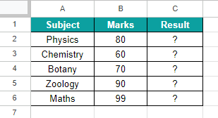
Now, let us learn how to find the rank of values in the data using RANK function formula with arrays.

The steps are:

Step 1: To begin with, we need to enter the data in the spreadsheet. In this example, the data is available in the cell range A1:C6. Next, select the cell where we want to find the result. In this example, we need to select the cell C2.

Step 2: Next, we need to insert the RANK function.

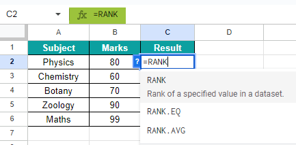
So, the complete formula is =RANK(B2,$B$2:$B$6)

Step 3: Press Enter key.

We will be able to see the result in cell C2, as shown in the below image.

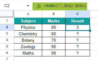
Now, using AutoFill option, we can find the result in the cell range C3:C6, as shown in the below image.

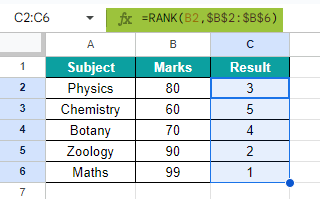
Likewise, we will be able to find the rank or position in Google sheets.

Example  #2 – RANK.EQ Function

RANK.EQ is a function similar to RANK function but assigns the same rank or position for the duplicate values in the data.

For example, consider the below table showing subject and marks in columns A and B, respectively.

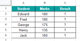
Now, let us learn how to find the rank of values in the data using RANK.EQ function formula in Google sheets.

The steps are:

Step 1: To begin with, we need to enter the data in the spreadsheet. In this example, the data is available in the cell range A1:C6. Next, select the cell where we want to find the result. In this example, we need to select the cell C2.

Step 2: Next, we need to insert the RANK function.

So, the complete formula is =RANK(B2,$B$2:$B$6)

Step 3: Press Enter key.

We will be able to see the result in cell C2, as shown in the below image.

Now, using AutoFill option, we can find the result in the cell range C3:C6, as shown in the below image.

Likewise, we will be able to find the rank or position in Google sheets using RANK.EQ function formula.

Example #3 – RANK.AVG Function

RANK.AVG is a function similar to RANK function and RANK.EQ functions but assigns the rank or position in the data based on the average.

For example, consider the below table showing subject and marks in columns A and B, respectively.

Now, let us learn how to find the rank of values in the data using RANK.AVG function formula.

The steps are:

Step 1: To begin with, we need to enter the data in the spreadsheet. In this example, the data is available in the cell range A1:C6. Next, select the cell where we want to find the result. In this example, we need to select the cell C2.

Step 2: Next, we need to insert the RANK.AVG function.

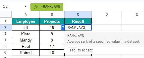
So, the complete formula is =RANK.AVG(B2,$B$2:$B$6)

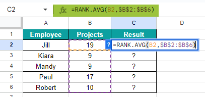
Step 3: Press Enter key.

We will be able to see the result in cell C2, as shown in the below image.

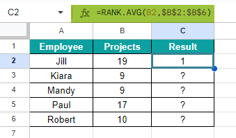
Now, using AutoFill option, we can find the result in the cell range C3:C6, as shown in the below image.

Likewise, we will be able to find the rank or position in Google sheets using RANK.AVG formula.

Important Things To Note

• Google sheets RANK function, in simple terms, ranks the data in ascending or descending order.
• It is an inbuilt function grouped under Statistical function category.
• Remember, the Google sheets RANK.EQ function ranks the data with same position if there are duplicate values.
• RANK function may not work if the data has any non-numeric data or textual values. It works only for numeric data.

Frequently Asked Questions (FAQs)

Recommeded Articles

Guide to What Is RANK Function In Google Sheets. We learn its formula and how to use it to find the rank of a value with step-wise examples0. You can learn more from the following articles. –

Organizational Chart In Google Sheets

RIGHT Function In Google Sheets

SUMPRODUCT With Multiple Criteria In Google Sheets