
What Is REDUCE In Google Sheets?
REDUCE function in Google sheets, as the name suggests, is used to apply a function to each array element to get a single output result. It is a default function in Google sheets and is mostly used in programming languages like python, java etc., Apart from programming languages, REDUCE function is also available in Excel. This function is mostly used to find the sum (total) or the product (multiplication) of an array.
For example, consider the below table showing values in column A and column B shows the total of the values.

Now, we can use the REDUCE function with SUM to find the result in Google sheets.
Use this REDUCE In Google Sheets Template to follow along with the examples in this article.
Download Excel TemplateTo begin with, we need to enter the data in the spreadsheet and select the cell where we want to find the result. Next, enter the REDUCE function formula, =REDUCE(0,A2:A6,LAMBDA(total,x,total+x)). Press Enter key.
We will be able to see the result in cell C2, as shown in the below image.

In this article, let us learn how to use REDUCE function in Google sheets with detailed examples.
Key Takeaways
- REDUCE function in Google sheets is a default function used to find the final rest by accumulating the values in the formula.
- The formula of REDUCE function in Google sheets is =REDUCE(initial_value,array_or_range,LAMBDA) where all three arguments are mandatory.
- Note that the initial_value is the reducing value. It is the accumulator and the first element in the array.
- Array_or_range shows the cell range which is reduced using the formula.
- LAMBDA is the function with two arguments – the current accumulator value and the current element of the array.
Syntax

The formula or syntax of REDUCE function in Google sheets is =REDUCE(initial_value,array_or_range,LAMBDA)
where,
- Initial_value is the mandatory argument for reducing the value. It is used as an accumulator and is the first element in the array.
- Array_or_range is also a mandatory argument showing the cell range which is reduced using the formula.
- LAMBDA is the function with two arguments – the current accumulator value and the current element of the array. Remember, the function returns the new accumulator value.
How To Use REDUCE Function In Google Sheets?
We can use the REDUCE function in Google sheets with two methods.
They are:
- Selecting the formula under the Insert tab
- Manually typing the formula
Method #1 – Selecting the formula under the Insert tab
The steps to select the REDUCE function formula under the Insert tab are:
Step 1: To begin with, we need to enter the data in the spreadsheet. Next, we need to select the cell where we want to find the result.
Step 2: Next, select the Insert tab and click on the Array group of functions.
Step 3: Then, click on the REDUCE function in Google Sheets. It is available in the list of available options, as shown in the below image.

Step 4: Now, we will be able to see the REPLACE function formula in Google sheets.
Now, we can add the arguments and press Enter key to find the result.
Likewise, we can use the REPLACE function in Google sheets under the Insert tab.
Method #2 – Manually typing the formula
The steps to select the REDUCE function formula manually are:
Step 1: To begin with, we need to enter the data in the spreadsheet. Next, we need to select the cell where we want to find the result.
Step 2: Next, enter =RE and click on the REDUCE function in the list of options, as shown in the below image.

Alternatively, we can manually enter =REDUCE directly in Google sheets.
Step 3: Now, we will be able to see the REPLACE function formula in Google sheets.
Now, we can add the arguments and press Enter key to find the result.
Likewise, we can use the REPLACE function in Google sheets manually.
Examples
Now, let us learn how to use the REDUCE function in Google sheets with the following detailed examples.
Example #1
For example, consider the below table showing data in column A and column B shows the total of the values.

Now, we can use the REDUCE function with SUM to find the result.
The steps are:
Step 1: To begin with, we need to enter the data in the spreadsheet. In this example, the data is available in the cell range A1:A6. Next, we need to select the cell where we want to find the result. In this example, we need to select the cell C2.
Step 2: Next, enter the REDUCE function formula in Google sheets with SUM function.
So, the complete formula is =REDUCE(0,A2:A6,LAMBDA(total,x,total+x)).

Step 3: Press Enter key.
We will be able to see the result in cell C2, as shown in the below image.

Likewise, we can use the REDUCE function with the SUM function.
Example #2 – Calculate The Sum Of Valuues in a Range
For example, consider the below table showing sample values in column A and column B shows the total of the values.

Now, we can use the REDUCE function with SUM to find the result.
The steps are:
Step 1: To begin with, we need to enter the data in the spreadsheet. In this example, the data is available in the cell range A1:A6. Next, we need to select the cell where we want to find the result. In this example, we need to select the cell C2.
Step 2: Next, enter the REDUCE function formula in Google sheets with SUM function.
So, the complete formula is =REDUCE(0,A2:A6,LAMBDA(total,x,total+x)).

Step 3: Press Enter key.
We will be able to see the result in cell C2, as shown in the below image.

Likewise, we can use the REDUCE function with the SUM function.
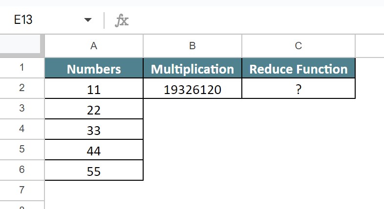
Example #3 – Multiply All The Values In A Range
For example, consider the below table showing data in column A and column B shows the multiplication of the values.

Now, we can use the REDUCE function with MULTIPLICATION to find the result in Google sheets.
The steps are:
Step 1: To begin with, we need to enter the data in the spreadsheet. In this example, the data is available in the cell range A1:A6. Next, we need to select the cell where we want to find the result. In this example, we need to select the cell C2.
Step 2: Next, enter the REDUCE function formula with MULTIPLICATION function.
So, the complete formula is =REDUCE(1,A2:A6,LAMBDA(multiply,x,multiply*x)).

Step 3: Press Enter key.
We will be able to see the result in cell C2, as shown in the below image.

Likewise, we can use the REDUCE function with the multiplication function.
Example #4 – Find The Maximum Value In A Range
For example, consider the below table showing value in column A and column B shows the maximum value.

Now, we can use the REDUCE function with MAX function to find the result.
The steps are:
Step 1: To begin with, we need to enter the data in the spreadsheet. In this example, the data is available in the cell range A1:A6. Next, we need to select the cell where we want to find the result. In this example, we need to select the cell C2.
Step 2: Next, enter the REDUCE function formula in Google sheets with SUM function.
So, the complete formula is =REDUCE(A2,A2:A6,LAMBDA(max, current, IF(current > max, current, max))).

Step 3: Press Enter key.
We will be able to see the result in cell C2, as shown in the below image.

Likewise, we can use the REDUCE function in Google sheets with the MAX function.
Important Things To Note
- REDUCE function in Google sheets requires all three arguments.
- Remember, we can combine REDUCE function with SUM, MAX, and MIN functions.
- Mostly, we can use the REDUCE function to find the total or product of an array.
Frequently Asked Questions (FAQs)
Now, we can use the REDUCE function with multiplication to find the result in Google sheets.
The steps are:
Step 1: To begin with, we need to enter the data in the spreadsheet. In this example, the data is available in the cell range A1:A6. Next, we need to select the cell where we want to find the result. In this example, we need to select the cell C2.
Step 2: Next, enter the REDUCE function formula in Google sheets with SUM function.
So, the complete formula is =REDUCE(1,A2:A6,LAMBDA(multiply,x,multiply*x)).
Step 3: Press Enter key.
We will be able to see the result in cell C2, as shown in the below image.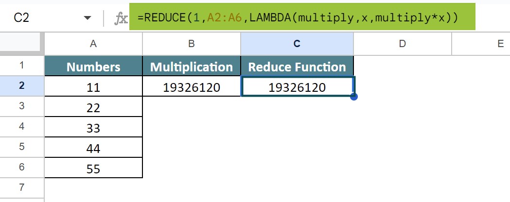
Likewise, we can use the REDUCE function in Google sheets with the multiplication function.
The REDUCE function may not work if one of three arguments are not included in the formula. Similarly, we might get an error when the data is not related with the arguments inputted in the formula.
Functions such as MAP, FILTER and REDUCE functions all work the same way. Especially, while using python programming language, we can use any of the function.
Use this REDUCE In Google Sheets Template to follow along with the examples in this article.
Download Excel Template