What is the RRI Excel function?
The RRI Excel (Rate of Return on Investment) function is a powerful tool used in financial analysis to calculate the equivalent interest rate for the growth of an investment. It provides a standardized measure of evaluating the profitability and performance of different investment opportunities. By using this function, we can determine the effectiveness of investments and make informed decisions.
The RRI Excel function considers the initial investment amount, final value, and holding period to provide a percentage rate that represents the growth over time.
To understand the RRI Excel function, let’s look at the formula below for 8 years, with a present value of 100 and a future value of 200. To begin, enter the following formula in cell B1:
=RRI(8, 100, 200)

The resulting value will be displayed in cell B1, as seen below. Thus, you can effortlessly grasp the returns on your investment.
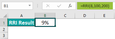
Table of contents
Key Takeaways
- The RRI Excel function helps calculate the expected return on investment. It considers factors like present value, future value, and the number of periods.
- RRI is highly valued by professionals for making informed investment decisions and evaluating different options based on their potential returns.
- With its ability to handle complex calculations quickly and accurately, the RRI Excel function has become an integral part of financial planning and decision-making processes in various industries.
Syntax

- Present Value (PV) – This refers to the initial worth of the investment as of the current date.
- Future Value (FV) – This signifies the ending value to which the investment has grown since the present date.
- Number of Periods (nper) – This represents the total number of compounding periods for an investment. It signifies the duration over which the investment will grow.
How To Use RRI Excel Function in Excel ?
To effectively utilize the RRI function in Excel, follow these steps.
#1 – Access from the Excel ribbon
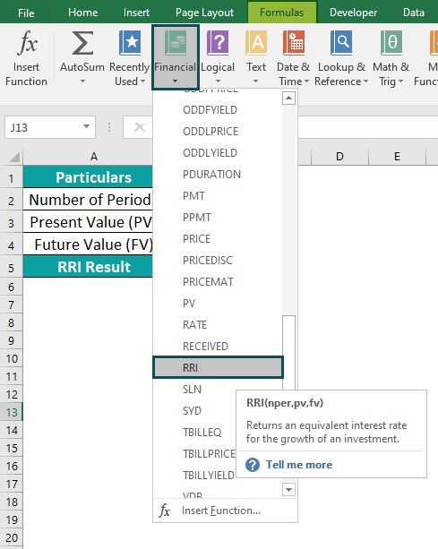
- Choose the empty cell which will contain the result. Go to the “Formulas” tab and click it.
- Select the “Financial” option from the list.
- Select “RRI Excel Function” from the drop-down menu.
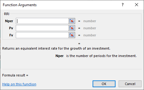
- A window called “Function Arguments” appears. Enter the value in the “Nper,” “Pv” and “Fv.” Select OK.
#2 – Enter the worksheet manually
- Select an empty cell for the output. Type “=RRI()” in the selected cell. Alternatively, type “=R” and double-click the RRI Excel function from the list of suggestions shown by Excel.

- Press the “Enter” key after entering the values for the arguments.

Examples
Example #1 – Calculating RRI Value for the Day Period
To gain a comprehensive understanding and apply the RRI Excel, let us delve into the following example:
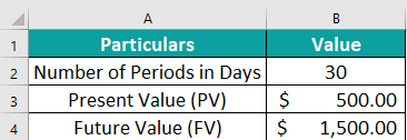
The data in the table is organized as follows.
- Row 2 contains the Number of Periods in days.
- Row 3 has the Present Value.
- Row 4 holds the Future Value.
To calculate the desired output, follow the steps below.
Step 1: Select the cell where the formula will be entered to compute the result. Here, let us choose cell B5. Proceed to enter the formula in cell B5. The formula to be entered is as follows:
=RRI(B2,B3,B4).
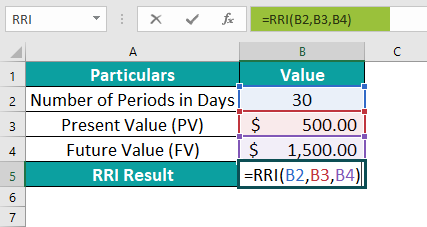
Step 2: Upon entering each value in column B, press the Enter key. The resulting value will be promptly displayed in cell B5, as seen below.

Example #2 – Calculating RRI Value For Monthly Period
Let us look at an example where we must find the RRI value for a monthly period using RRI Excel.
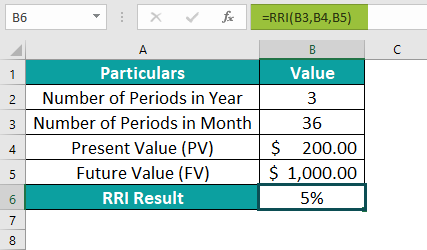
In the table provided, Row 3 shows the number of periods in Months. By multiplying the number of years by 12 (i.e., the number of years by the monthly adjustment factor), the total number of periods comes to 36. Row 4 displays the Present Value and Row 5, the Future Value. Row 6 reveals the RRI result. To calculate the desired output, follow these steps:
Step 1: Choose the cell where you want the formula and result to appear. For this demonstration, let’s go with cell B6.

Step 2: Enter the formula in cell B6. The complete formula to be entered in cell B6 is as follows:
=RRI(B3,B4,B5).
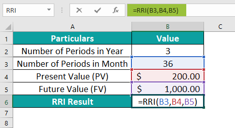
Step 3: After entering each value, enter the formula and press Enter. The resulting value will be promptly displayed in cell B6, just like in the image provided.
Example #3 – Calculating RRI Value For Quarterly Period
To effectively utilize the RRI Excel function for calculating quarterly results, let’s dive into this example:
In this organized table, the data is presented as follows:
- Row 2 showcases the periods in years.
- Row 3 exhibits the number of periods in Quarterly. By multiplying the number of years by 4, we get 16 periods, as shown in cell B3.
- Row 4 displays the Present Value.
- Row 5 represents the Future Value.
- Row 6 unveils the RRI result.
Now, let’s calculate the desired output by following these simple steps:
Step 1: Choose the cell where you want the formula and the result to appear. For this demonstration, let’s go with cell B6.
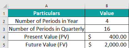
Step 2: Let us enter the formula in cell B6. The complete formula to be entered is as follows:
=RRI(B3,B4,B5).

Step 3: After entering each value in the previous step, hit the Enter key. The resulting value will be displayed in cell B6, just like in the image provided below.

Example #4 – Calculating RRI Value For Half-Yearly Period
To make use of the RRI Excel function for calculating half-yearly results, let’s dive into this example:
In this organized table, the data is presented as follows:
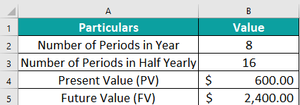
Here since in a year, we have 2 half-yearly periods each, for 8 years we have a total of 16 periods. Now, let’s calculate the desired output by following these simple steps.
Step 1: Select the cell to enter the formula and the result to appear. In this case, it would be cell B6. Enter the formula shown below into B6.
=RRI(B3,B4,B5).
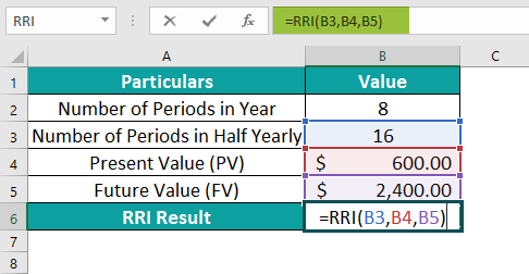
Step 2: Once you’ve entered each value in Column B, hit the Enter key. The resulting value will pop up in cell B6, just like in the image below.

Example #5 – Calculating RRI Value For Yearly Period
To better understand how to utilize the (Rate of Return on Investment) RRI Excel function for calculating yearly results, let’s delve into this example.
In this well-organized table, the data is presented as follows:

To calculate the desired output, we will follow these simple steps:
Step 1: Select the cell where you want the formula and the result to be displayed. For this demonstration, we will use cell B5. Enter the below formula in B5.
=RRI(B2,B3,B4).

Step 2: Once you have entered each value, simply press the Enter key. You will then see the resulting value promptly displayed in cell B5, just like in the image provided.

Important Things To Note
- The RRI Excel formula allows professionals to compare various projects or investments based on their potential returns and select the most beneficial option for their organization or clients.
- Error #NUM! – It occurs when either the nper or the pv argument is set to zero or when any of the supplied arguments are negative.
- Error #VALUE! – It occurs if any of the supplied arguments are non-numeric.

Frequently Asked Questions (FAQs)
The RRI Excel function calculates the rate of return for an investment by considering the initial investment, periodic cash flows and the number of periods. This valuable financial tool allows professionals to determine the growth rate needed to reach a desired future value. The formula behind RRI is based on compound interest calculations, enabling users to assess whether an investment opportunity is financially viable or not.
To better understand how to utilize the Rate of Return on Investment (RRI) function for calculating annual results, let’s delve into this example.
The formula enter in cell B5 is as follows: =RRI(B2, B3, B4). The calculated value will be shown in cell B5, as shown below.
The RRI function in Excel is a powerful tool for analyzing investment returns and interest rates, but it does come with certain limitations and constraints.
Firstly, the function assumes a constant rate of return over the entire period, which may not be realistic in many investment scenarios.
• Additionally, RRI requires that the cash flows be evenly spaced, meaning that irregular payment schedules cannot be accurately modeled.
• Another limitation is that RRI does not consider external factors such as inflation or market volatility, which can significantly impact investment returns.
• Furthermore, the function assumes that all cash flows occur at the end of each period and ignores any interim cash flows.
• Lastly, RRI may provide misleading results if used to compare investments with different timeframes or when comparing investments with differing risk levels.
One can activate the RRI function in Excel using the following steps:
• Go to the “Formulas” tab and click it.
• Select the “Financial” group.
• Select “RRI” from the drop-down menu.
• A window called “Function Arguments” appears.
• As the number of arguments, enter the value in the “Nper,” “Pv” and “Fv.”
• Select OK.
Download Template
This article must help understand the RRI Excel Function’s formula and examples. You can download the template here to use it instantly.
Recommended Articles
Guide to RRI Excel Function in Excel. Here we learn how to use RRI Excel Function in excel with step by step examples and a downloadable template. You can learn more from the following articles –

Leave a Reply