
What Is Structured References In Excel?
Structured References in Excel show a cell referenced using the Excel table and column names. And these references adjust automatically on data modification in the dataset.
Excel Structured References enables us to create dynamic formulas inside and outside the Excel tables. And they help locate Excel tables in large workbooks quickly.
Use this Structured References In Excel Template to follow along with the examples in this article.
Download Excel TemplateFor example, the table below shows a student’s scores in five subjects. Cell B8 shows the sum of all the subject scores using the SUM excel function with the relative reference to the required cell range.

First, we will convert the above data range into an Excel table named Score_Table. And then, determine the sum of the subject scores using the Structured References to the cell range containing the scores in the SUM() in the target cell.
- Enter the formula =SUM(B2:B6) in cell B8.
- Enter the formula =SUM(Score_Table[Score Out Of 100]) in cell F8.
- Press “Enter” after entering the formula.

The output is “478”, as shown above, in cells B8 and F8. Therefore, in cell F8, we entered a formula using the table and column names to create the required Structured References in the SUM().And in cell B8 we entered the formula using the cell references. Cells B9 and F9 are for our reference.
We can enter the function and select the relevant table and column names from the drop-down lists that Excel suggests to perform the required calculations. Otherwise, we can click the Excel table cells we require to reference in the formula. Thus, the Structured References do not require us to type the cell references in the formulas.
Key Takeaways
- Structured References in Excel use the Excel table and column names for referencing the selected cells in place of the cell addresses.
- The Structured References adjust dynamically according to the changes in the Excel table, and one can utilize them inside and outside the Excel table. Thus, the users can use this reference type in dynamic formulas and quickly locate Excel tables in worksheets.
- Suppose we enter a formula containing the Structured References in a cell. Then, we can use the AutoCorrect Options button to automatically copy the formula in the remaining cells of the same column to perform the same calculations.
How To Create Structured References In Excel?
The steps to create Structured References in Excel are as follows:
First, let us convert the data range into an Excel table. So, click on a cell in the data range (or select the entire data range), and follow the path Insert → Table, or press the shortcut keys Ctrl + T.
Next, the steps to obtain the Structured References in Excel table formulas are as follows:
- Select the target cell, enter the ‘=’ sign, the required function name, and open brackets.
- Enter the reference by selecting the required cell or cell range in the Excel table. Excel will show the respective column names as Structured References to the chosen cell or cell range.
- Close the brackets, and press Enter.
[Note: When we use the Structured References in Excel table formulas, Excel automatically fills the formula entered in one cell in the remaining cells in the column. Otherwise, we can click the AutoCorrect Options button, which appears after we enter the formula in one target cell in the Excel table. It will show the option to update the formula in the remaining cells in the column.
Furthermore, the formula in each target cell will remain the same. But Excel will use the corresponding row data to complete the calculation in each target cell.]
On the other hand, if we must enter the formula outside the Excel table. Then, the steps to create Structured References in such a scenario are as follows:
- Select the target cell, enter the ‘=’ sign, the required function name, and the opening parenthesis.
- We must enter the Excel table name. Once we type the first letter of the name, Excel will show the table names and inbuilt functions starting with the entered alphabet. We can then double-click on the required table name.
- Enter the opening bar bracket, followed by the reference, by selecting the required cell or cell range in the Excel table. Excel will show the respective column names as Structured References to the chosen cell or cell range.
- Next, enter the closing bar bracket. Follow steps 2 to 3 each time we wish to create Structured References to a cell or cell range in the formula.
- Finally, enter a close parenthesis to complete the formula, and press Enter.
But if we require only one cell range from the table, click on the formula expression after entering the Excel table name, and press the Tab key to execute the function.
Basic Example
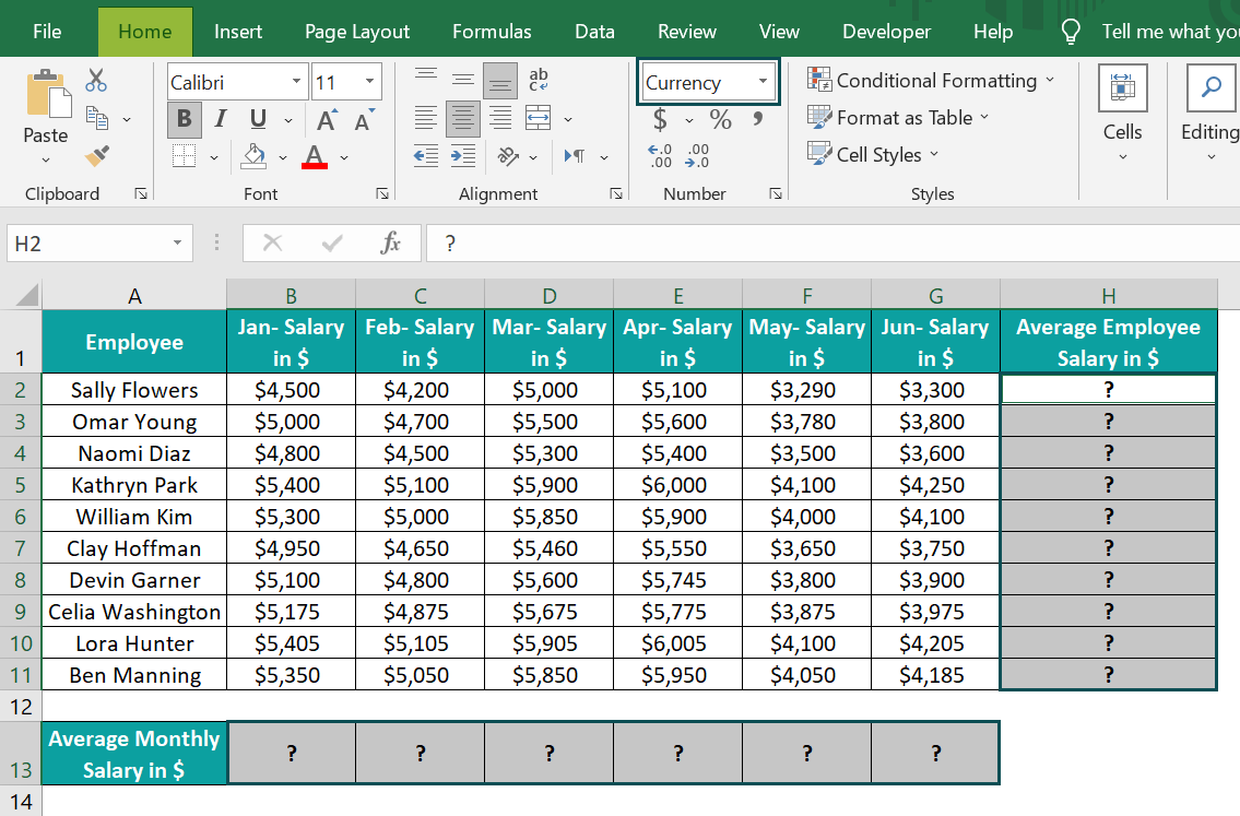
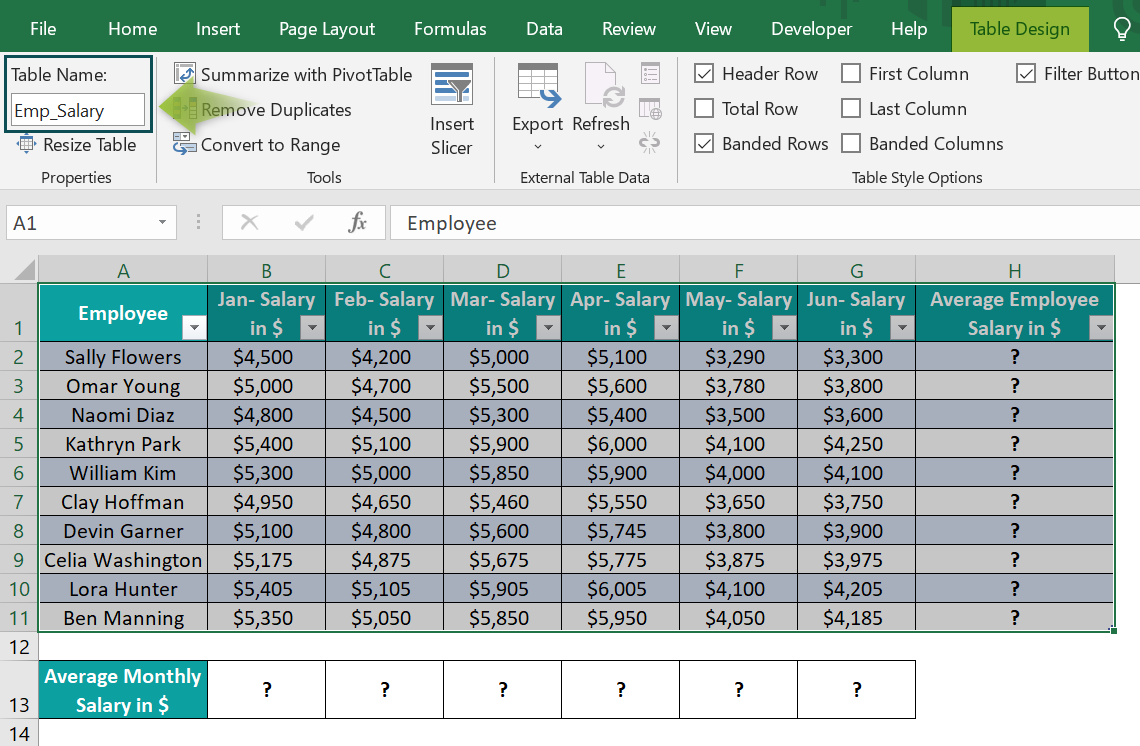
Let us determine the average employee salary in column H and the average monthly salary in row 13 using the Structured References Excel example.
The table below contains the monthly salary of ten employees from Jan-Jun.

The steps to form the absolute Structured References in Excel table formulas and the Structured References outside the Excel table are:
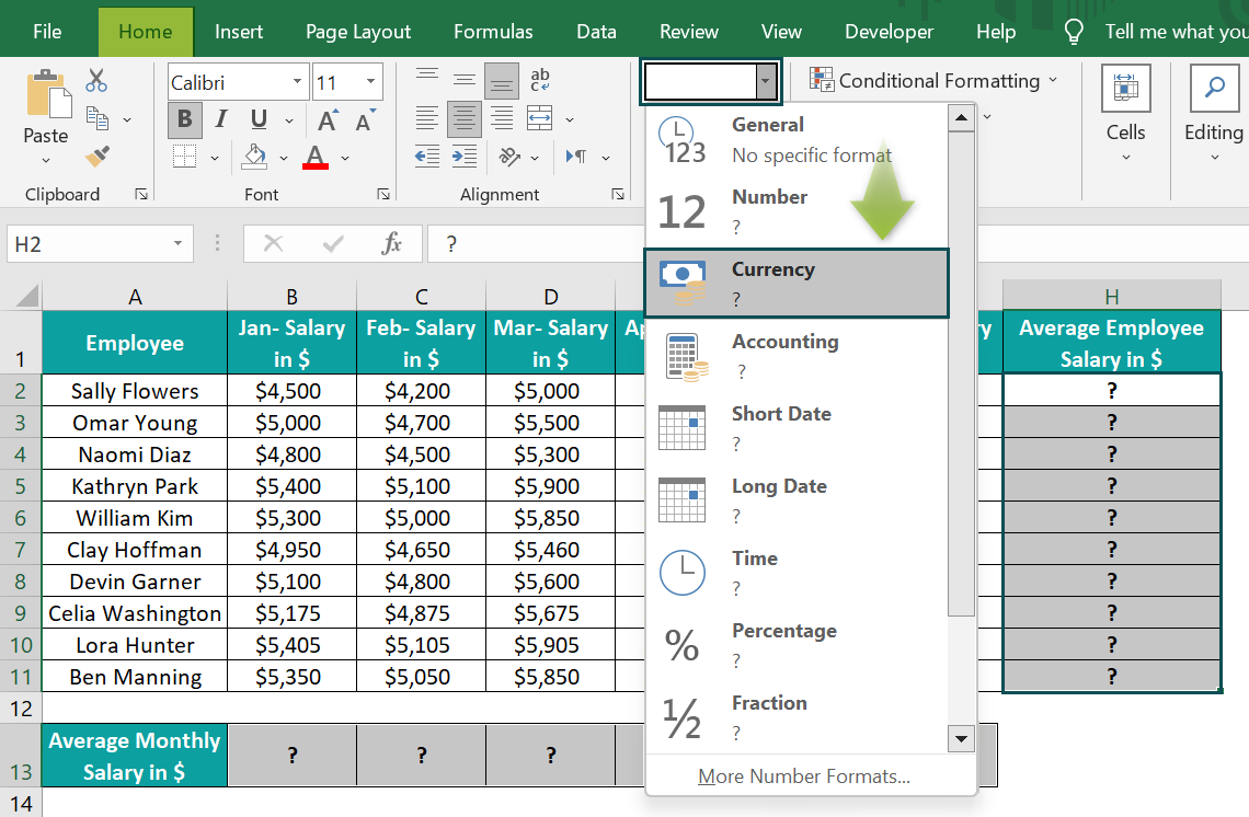
- Select the cell range H2:H11 and B13:G13, and set the data format in Home → Number Format as Currency.


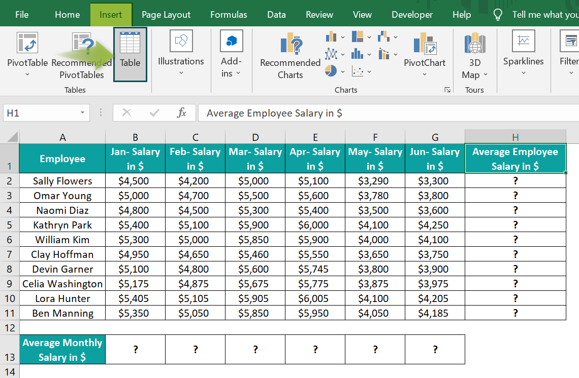
- Click on a cell in the data range A1:H11, and follow the path Insert → Table, or press the keys Ctrl + T, to convert the chosen data range into an Excel table.
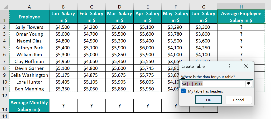
The Create Table window opens, showing the data range to convert into an Excel table. Ensure the table headers option remains selected.
- Click OK to get the required Excel table with the Design tab open. Update the Table Name field in the Design tab as, say, Emp_Salary.
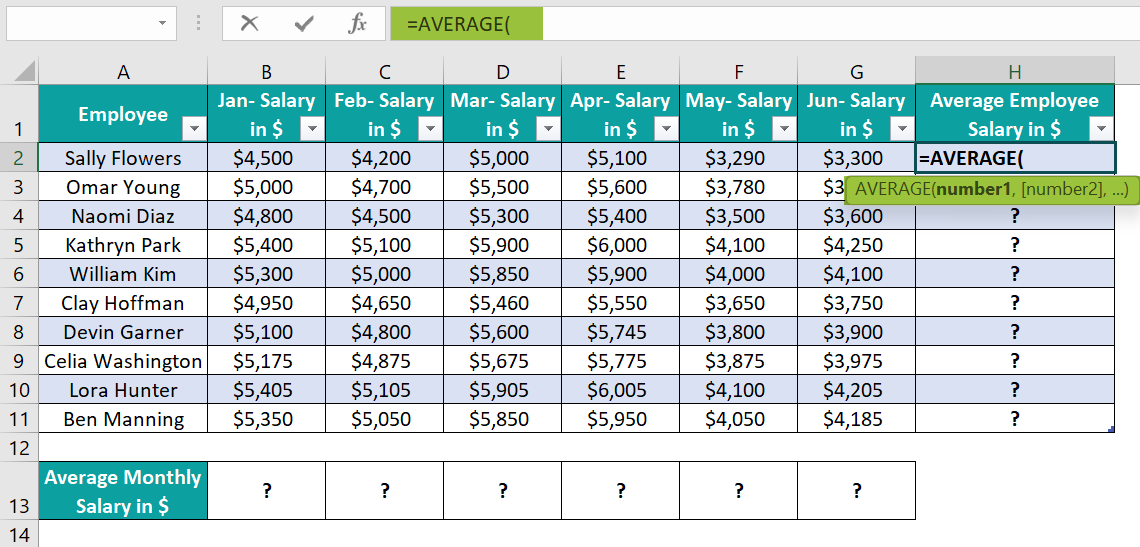
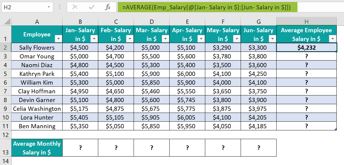
- Select cell H2, and entering the AVERAGE() formula =AVERAGE(

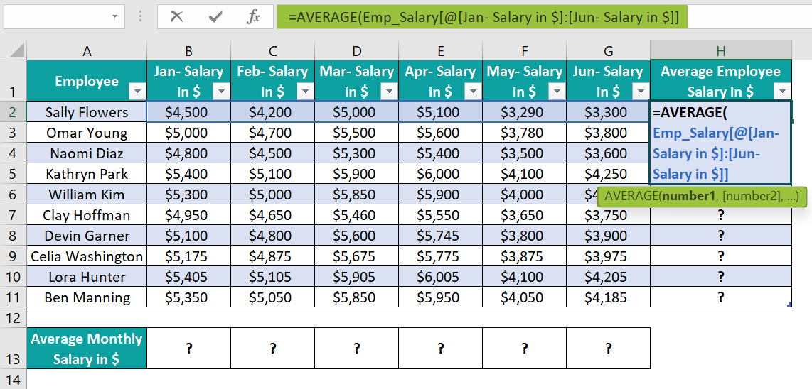
To find the average employee salary, select the cell range from B2:G2, which will create the Structured References in the AVERAGE(), showing the table and column names for the chosen cell range.
=AVERAGE(Emp_Salary[@[Jan- Salary in $]:[Jun- Salary in $]]
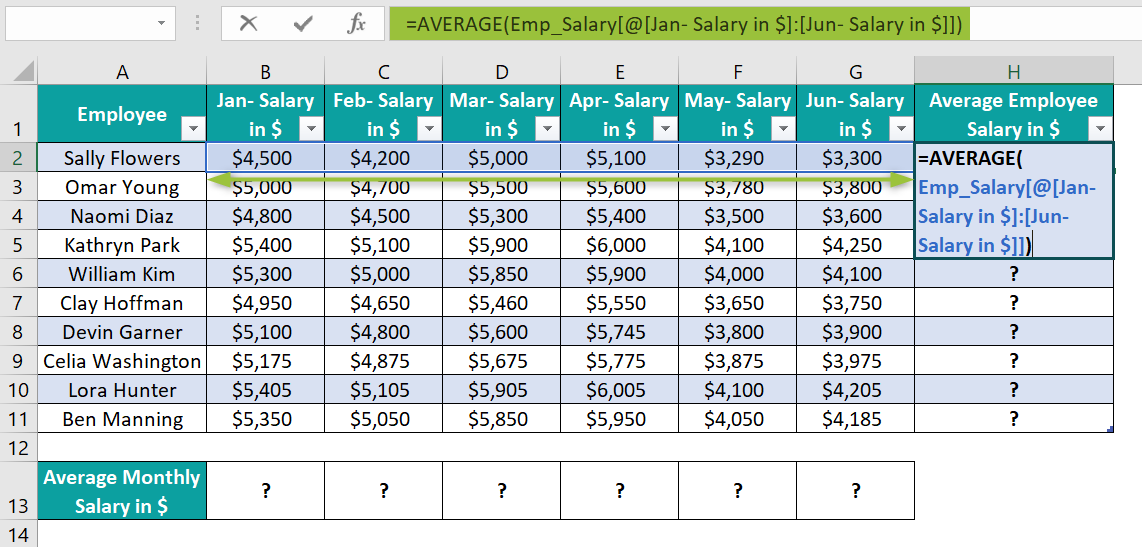
Next, close the brackets, =AVERAGE(Emp_Salary[@[Jan- Salary in $]:[Jun- Salary in $]])
- Press Enter to view the average salary of Sally Flowers in cell H2.

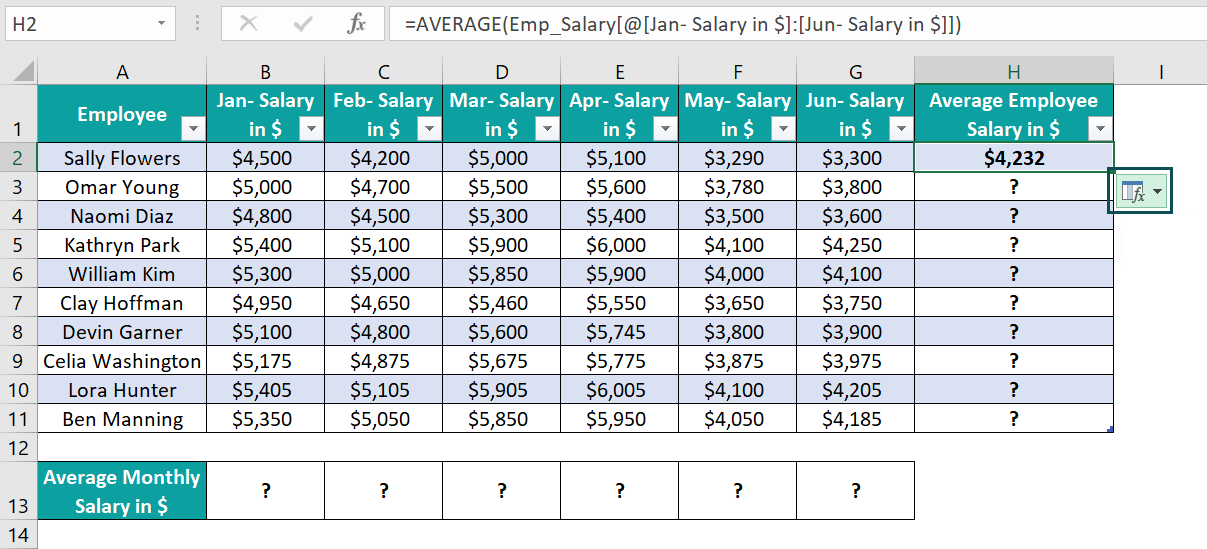
- Hover on the AutoCorrect Options button.

And click the down arrow in the button and the overwrite option to auto-fill the absolute Structured References in Excel table formulas in cells H3:H11.
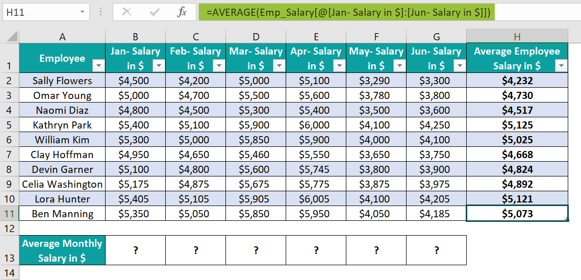
When we enter the formulas containing the Structured References in the Excel table, the Structured References are absolute by default, as shown below.
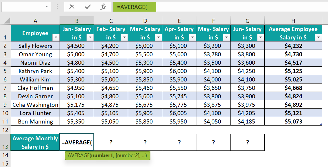
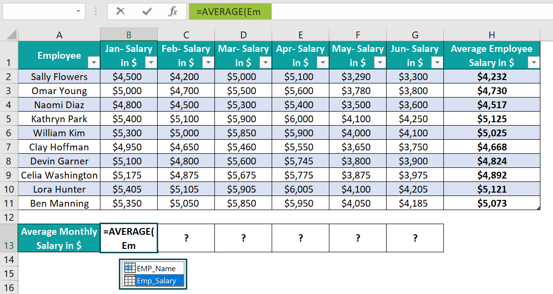
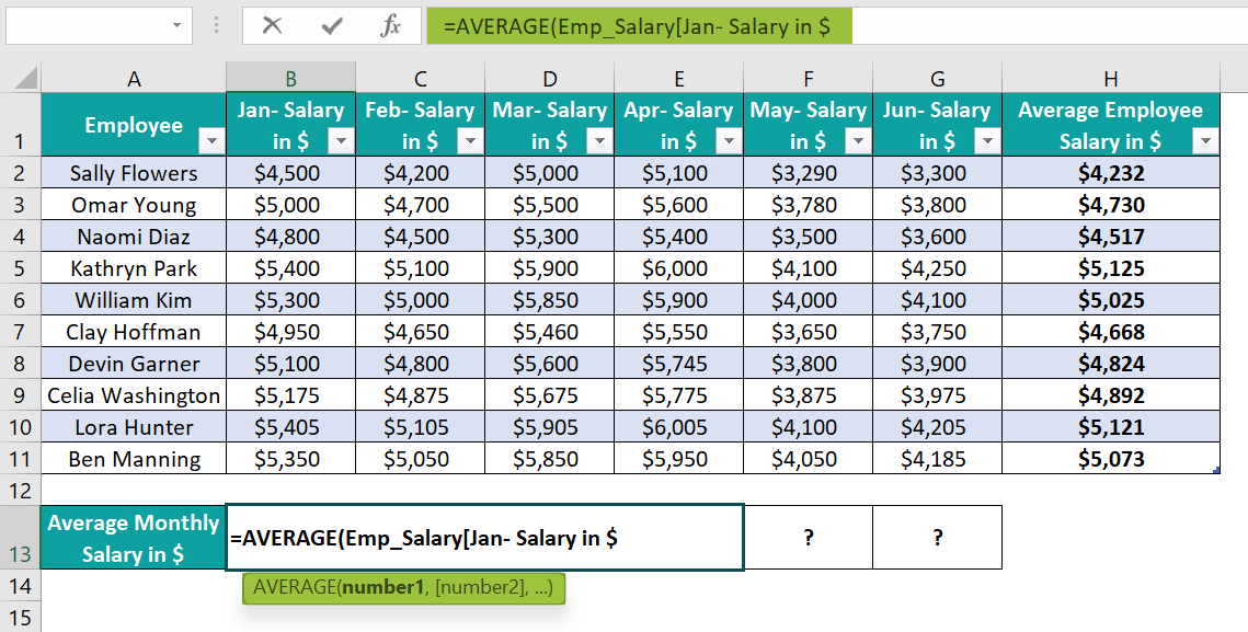
- Select cell B13, and enter the AVERAGE() formula =AVERAGE(

Next, as we set the Excel table name as Emp_Salary, enter the text “Em”. Excel will show a list of table names starting with the entered characters, i.e.,
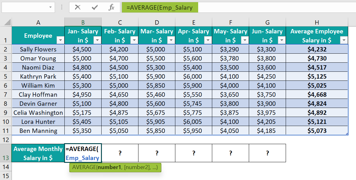
=AVERAGE(Em, and double-click on the table name Emp_Salary to choose it.
And click cell B13 expression, i.e., =AVERAGE(Emp_Salary
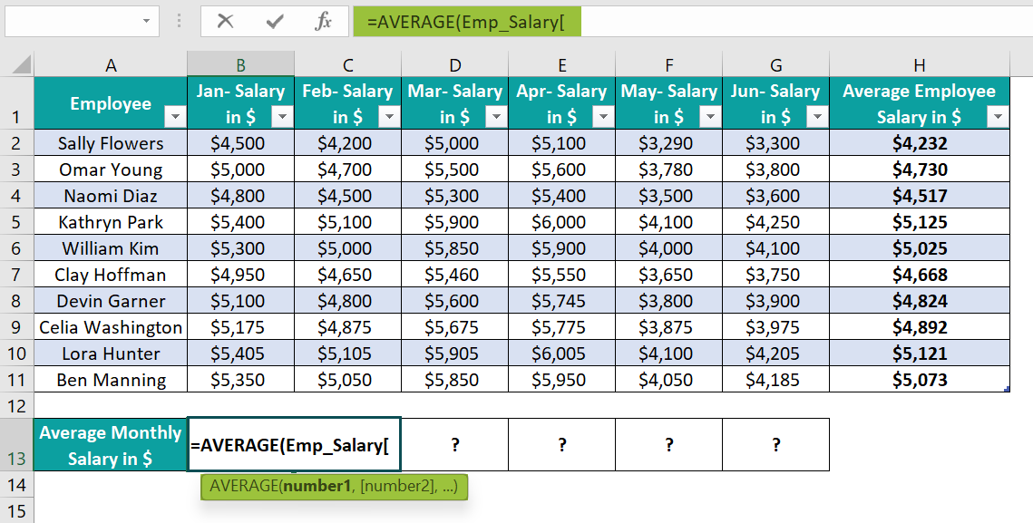
Next, enter the opening bar bracket =AVERAGE(Emp_Salary[
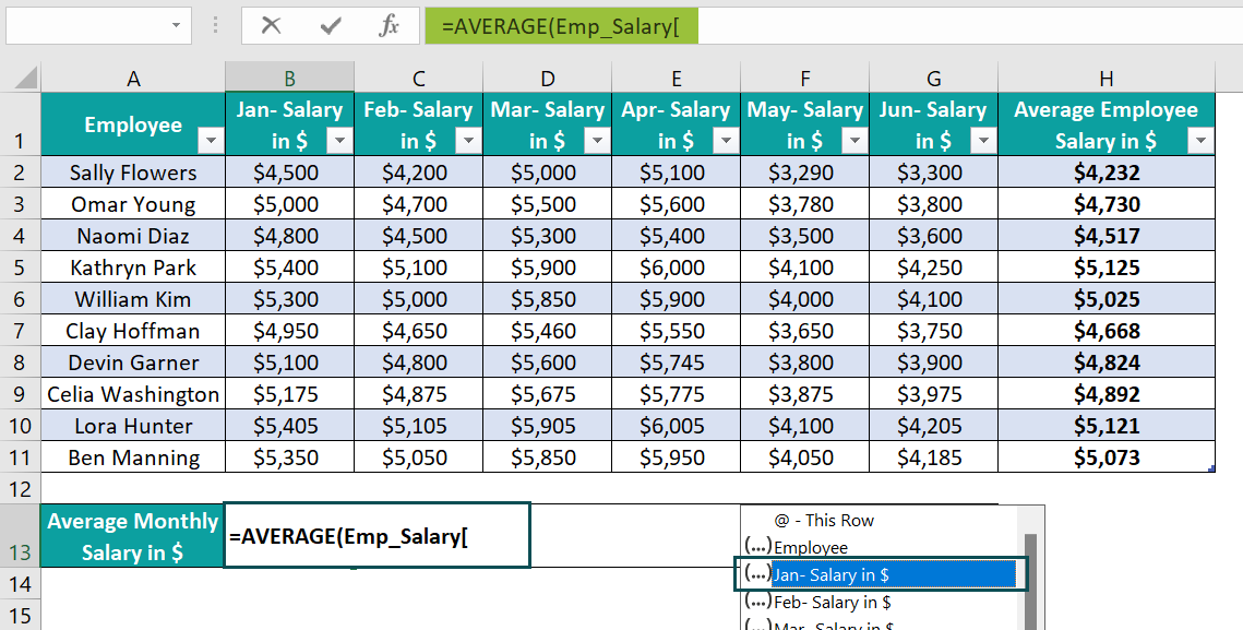
Excel will show a list of column headings from the Emp_Salary Excel table. And as we require the average monthly salary in Jan, double-click on the Jan- Salary in $ column heading option.
=AVERAGE(Emp_Salary[Jan- Salary in $
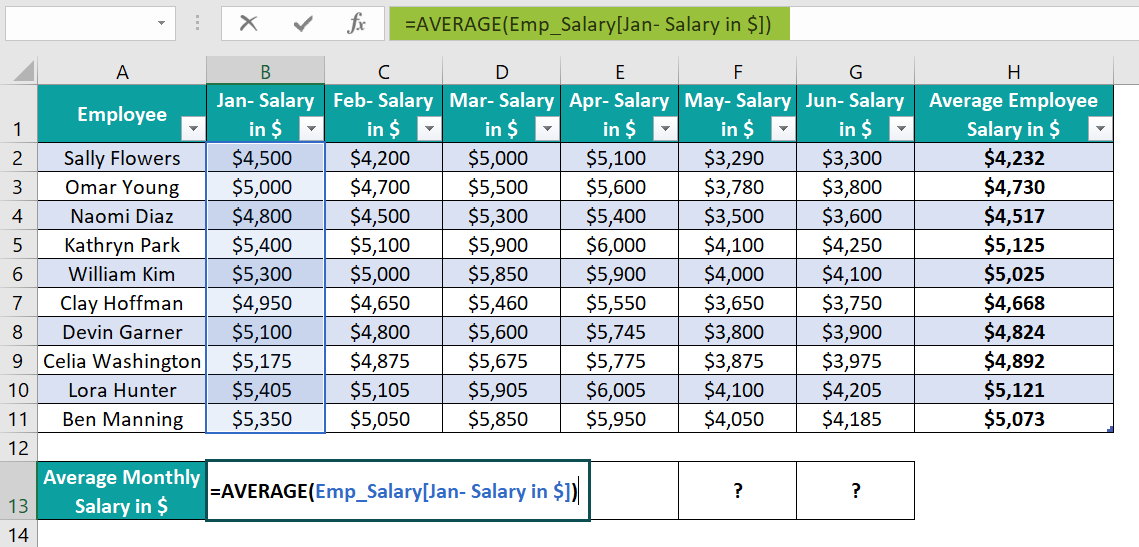
Next, enter the closing bar bracket and parenthesis to complete the formula.
=AVERAGE(Emp_Salary[Jan- Salary in $])
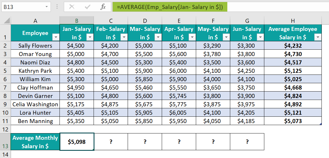
- Press Enter to execute the formula and obtain the average salary in January.
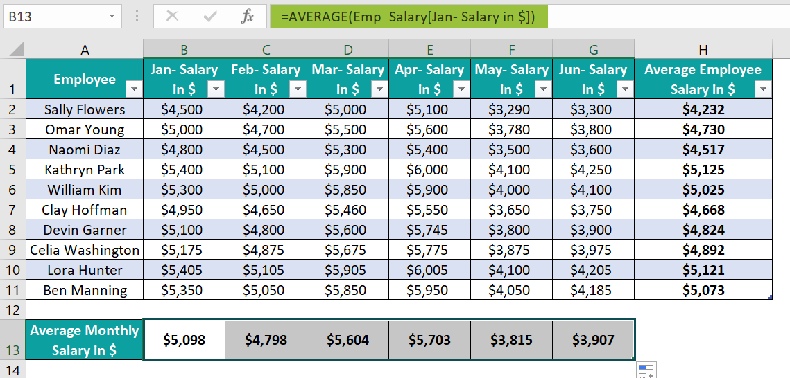
- Using the fill handle, drag the formulas to cells C13:G13.

The formulas in cells C13:G13 contain relative Structured References.
Furthermore, the formulas in the cell range H2:H11 are the same as the data range to calculate the average salary of each employee in each target cell is the same.
On the other hand, as the column range to determine the average salary for each month differs, the formulas in the target cells in the range B13:G13 are different.

Examples
Check out the following illustrations of Excel Structured References to use the feature effectively.
Example #1
The table below shows the sales data for five branch offices of a firm. We must determine the lowest sales figures based on the given data using Structured References.

The steps to enter Excel Structured References are as follows:
- Step 1: Click cell range A1:B6, and follow the path Insert → Table to convert the chosen data range into an Excel table.

The Create Table window will open, where we can see the selected data range reference.

Click OK to view the Excel table.

- Step 2: Click a cell in the Excel table to enable the Design tab, and update the Table Name field as BO_Sales.

- Step 3: Select cell B8, and type the MIN excel formula =MIN(

Next, according to the Structured References Excel definition, we must type the first or first few letters of the Excel table name, BO.

Excel shows the table names starting with BO as a drop-down list.

Double-click on the required table name, BO_Sales, i.e., =MIN(BO_Sales

Next, click cell B8 expression, and enter an opening bar bracket as =MIN(BO_Sales[

Excel will display a drop-down list of column names from the Excel table BO_Sales and a few other options to use the BO_Sales table data.
As we require the lowest sales figures based on column B data in the BO_Sales table, double-click the corresponding column name, Sales in USD, to select it.
=MIN(BO_Sales[Sales in USD

And then, enter a closing bar bracket and parenthesis to complete the formula.
=MIN(BO_Sales[Sales in USD])

- Step 4: Press Enter to view the output in cell B8, $10,000.

The MIN() checks the values in the data range specified by the Structured References and returns the lowest value from the list to display in the target cell.
Example #2
The following table shows the quantities of fruits delivered each year from 2018-22. We will find the total years of data available for each fruit in column G using Structured References in Excel.

The steps to use the Structured References are as follows:
- Step 1: Click on a cell in the given data range, and press Ctrl + T to open the Create Table window.

Clicking OK will convert the chosen data range into an Excel table with the Design tab enabled.

- Step 2: Update the Table Name field as Item_Table in the Design tab.

- Step 3: Select cell G2, and type the COUNT excel formula =COUNT( as it counts the cells containing numbers in a cell range.

Next, select the cell range B2:F2, as we must count the total cells containing numbers in the specified range. =COUNT(Item_Table[@[2018 (Boxes)]:[2022 (Boxes)]]

Then, close the brackets as, =COUNT(Item_Table[@[2018 (Boxes)]:[2022 (Boxes)]])

- Step 4: Press Enter to view the required count in cell G2.

- Step 5: Hover on the AutoCorrect Options icon. And using its down arrow, click the option to overwrite the cells in column G with the COUNT().


Choosing the above-mentioned option will auto-fill cells G3:G6 with the required counts in the respective target cells based on the corresponding rows’ data.

Problems With Excel Structured References
Structured References help understand the formulas quickly. However, users may face issues while using them in practical scenarios. We shall see the two most common problems with Structured References.
Problem #1
Consider the table below containing monthly expenses and savings data.

The steps to calculate the total expenses and savings at the end of the respective columns, first, we will convert the data range into an Excel table are:
- Step 1: Click on a cell in the data range and press Ctrl + T to open the Create Table window.

Clicking OK will give us the required Excel table, where we must right-click to open the context menu. Select Table → Totals Row.

- Step 2: The above-mentioned action will insert a Total row at the bottom of the Excel table, with the last column total displayed.

Delete the last column total.

- Step 3: Select cell D9, click the down arrow button, and select Sum.

The above step gives the total monthly expense value in cell D9 by applying the formula:
=SUBTOTAL(109,[Monthly Expenses in $])

The formula returns the sum of the values in the visible rows of column D.
On the other hand, entering a row for displaying the total values and applying the formula SUM([Monthly Expenses in $]) manually in cell D9 will result in a circular reference. And the output will be $0. However, manually entering the formula SUM(D3:D8) will work and give the same output, $2,210.
Furthermore, the SUM() will add the data in hidden and visible rows in column D to return the required sum value.
- Step 4: As we require the total monthly savings in cell E9, select cell D9 and press Ctrl + C to copy the cell formula.

Next, select cell E9 and press Ctrl + V to paste the cell D9 formula.

The Structured References do not change with the cell when we copy the formula from one cell into another. And we obtain the total monthly expenses value in cell E9 as well. It is an issue with Structured References.
On the other hand, this does not happen when we enter a formula with a relative cell reference. We would see the cell references updating with changing target cells.
But the solution to the above problem is to select cell D9 and drag the excel fill handle to enter the formula in the remaining target cells, in this case, cell E9.


We can now see that the Structured References are there in the monthly savings column data in the cell E9 formula. And the function returns the correct total monthly savings, $3,230.
Problem #2
The table below shows the quarterly sales of a set of products.

The steps to calculate the total sales of Desktops in each quarter using Structured References, and display the outcome in cells C15:F15 are,
- Step 1: Click on a cell in the data range, and press Ctrl + T to open the Create Table window.

Click OK to obtain the required Excel table.

- Step 2: Clicking a cell in the Excel table or selecting the entire Excel table will show the Design tab in the Ribbon. Update the Table Name field as Quarterly_Sales in the Design tab.

- Step 3: Select cell C15 and start entering the SUMIF() as =SUMIF(

Next, to enter the range, type Q so that Excel shows the drop-down list of table names and functions starting with Q. Double-click on the Quarterly_Sales table name.

=SUMIF(Quarterly_Sales

Enter the opening bar bracket. Excel will show the Excel table column names to choose the required column data. As we must search Desktop in the Product column, we shall double-click the column name Product to select it.

The formula becomes: =SUMIF(Quarterly_Sales[Product

Next, we must enter the criteria. It is the absolute reference to cell B15, which contains the product for which we require the quarterly total sales values.
So, enter a closing bar bracket, a comma, $B$15, and a comma as,
=SUMIF(Quarterly_Sales[Product],$B$15,

Next, we must provide the sum_range. And for that, we should type the letter Q to select the table name, as explained earlier, and enter an opening bar bracket.

=SUMIF(Quarterly_Sales[Product],$B$15,Quarterly_Sales[
Entering the opening bar bracket will show the drop-down list of columns in the Excel table.
As we require Q1 total sales data, double-click the column name, Q1- Sales in $, to select it.

=SUMIF(Quarterly_Sales[Product],$B$15,Quarterly_Sales[Q1- Sales in $

Next, enter the closing bar bracket and parenthesis to complete the formula.
=SUMIF(Quarterly_Sales[Product],$B$15,Quarterly_Sales[Q1- Sales in $])

- Step 4: Press Enter to view the Q1 total sales of Desktop in cell C15.

- Step 5: Using the fill handle, implement the formula in cells D15:F15.

But the issue is that the Structured References in the formula copied cause the formula to return incorrect values in cells D15:F15.

The reason is that the relative Structured References in the range argument change with each target cell. But we require the range argument to remain the same in all the target cells. So, we should provide the absolute Structured References to the Product column in the range argument.
Here is how to modify the cell C15 formula.
Enter a bar bracket after the table name and a colon (‘:’) after the term [Product] in the range argument. And enter an opening bar bracket, which will show the drop-down list of the Excel table columns. Double-click on the Product column name to select it. And enter two closing bar brackets to complete the formula.

The formula is =SUMIF(Quarterly_Sales[[Product]:[Product]],$B$15,Quarterly_Sales[Q1- Sales in $])

- Step 6: Press Enter to view the output in cell C15.

- Step 7: Using the fill handle, update the formula in cells D15:F15.


Thus, the range argument value remains the same in all the target cells. And the column to add the sales values in each quarter for Desktop must vary accordingly. So, the sum_range argument includes relative Structured References to the corresponding column in each target cell formula.
Thus, we get the correct Desktop’s total sales value in each quarter in cells C15:F15.
For example, the SUMIF() in the cell F15 formula checks for cells containing the product Desktop in the Product column. The item is in cells B4, B7, and B11. And thus, the function adds the values in the same rows but in the Q4- Sales in $ column (cells G4, G7, and G11) to return the Q4 total sales value of $6,595.
How To Turn Off Structured References In Excel?
The steps to turn off Structured References in spreadsheets are as follows:
- Step 1: Click File → Options to open the Excel Options window.


- Step 2: Open the Formulas tab in the Excel Options window.

- Step 3: Uncheck the option Use table names in formulas in the Working with formulas section in the Formulas tab, and click OK, as shown below.

Important Things To Note
- Ensure to enter the column name twice, separated by a colon, to create an absolute Structured References.
- When applying a cell formula containing Structured References in adjacent cells in the same row, drag the fill handle to update the formula in the required cells.
- If the Excel table column names include spaces or special characters, then the Structured References in Excel will include an additional bar bracket set to enclose such column names.
- Ensure to turn off the Structured References option in the Excel Options window if we wish not to use it in our spreadsheet.
Frequently Asked Questions (FAQs)
We can use the IF and Structured References in Excel in the following way. Let us see the steps with an example.
The below table contains the students’ scores in four subjects.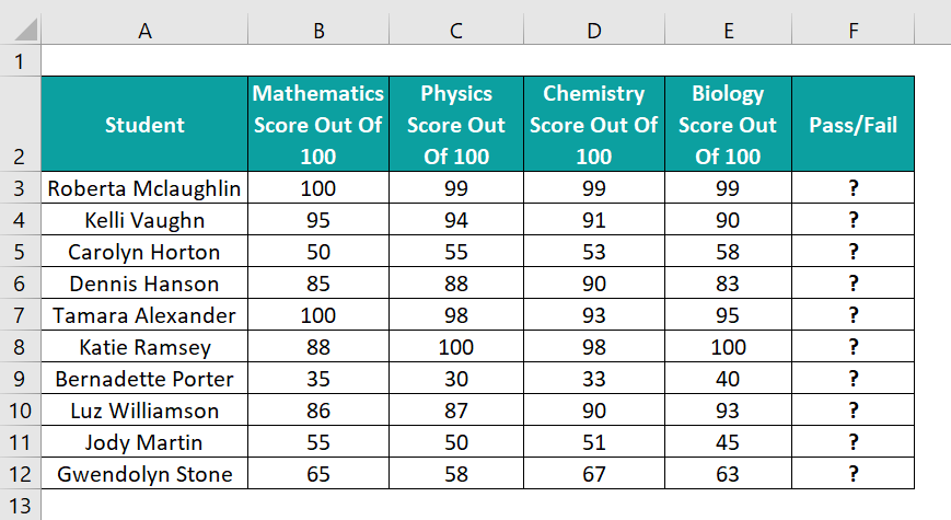
Suppose the requirement is to determine the pass status of each student based on their aggregate of the four subjects. Assume the cutoff to pass a student is an aggregate of 250, and we must display the status in column F.
Then, here is how to use the Structured References in the IF() in the target cells and achieve the desired information.
• Step 1: Click on a cell in the given data range, and press Ctrl + T to open the Create Table window.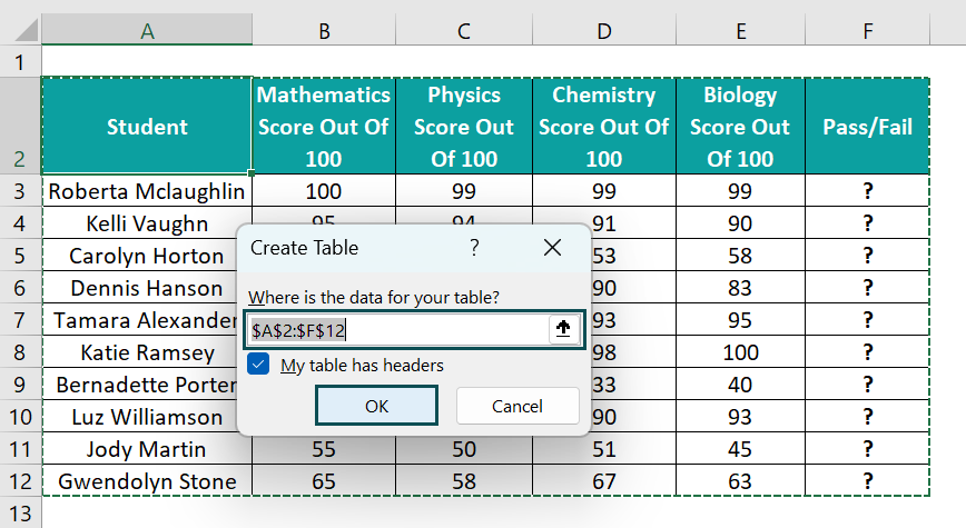
Clicking OK will result in the following Excel table, with the Design tab visible in the Ribbon.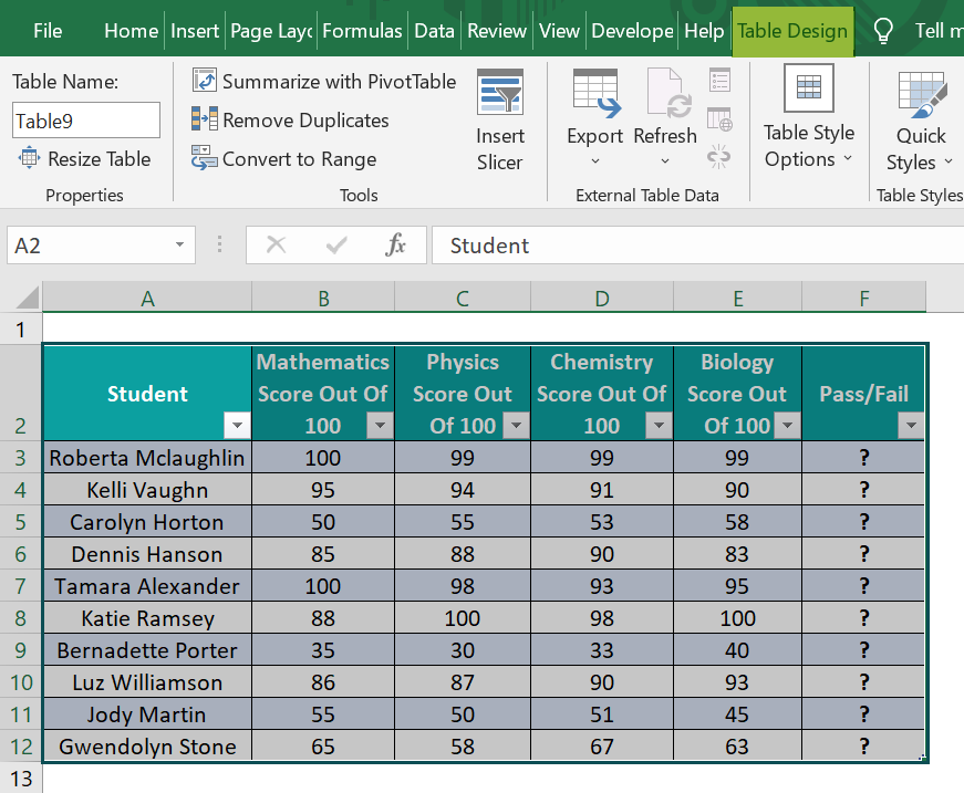
• Step 2: Let the Excel table remain selected to keep the Design table visible, and update the table name in the Design tab as Subject_Scores.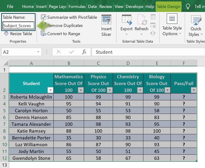
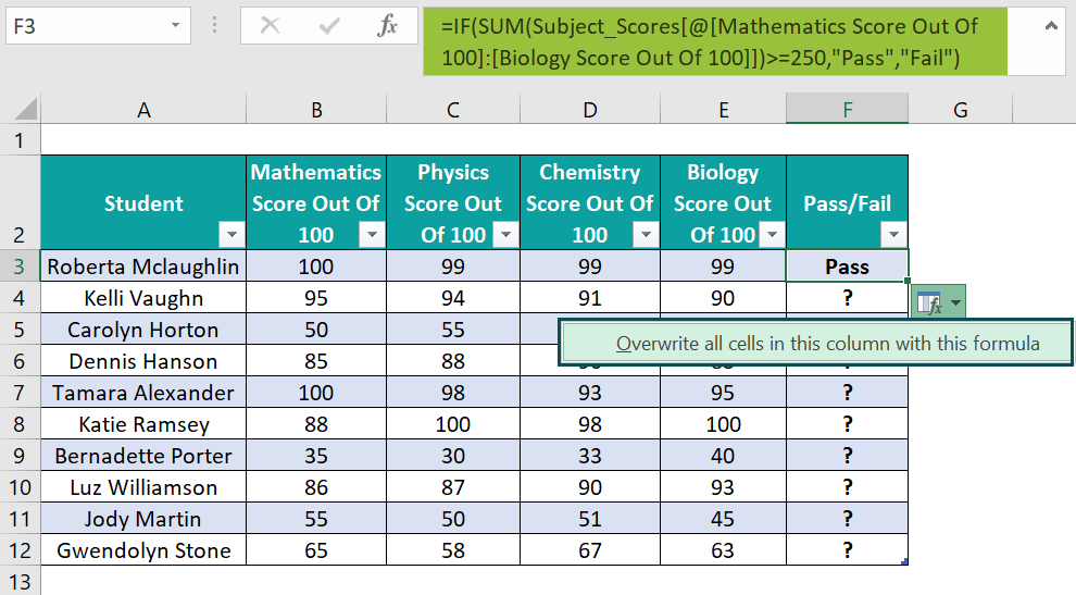
• Step 3: Select cell F3 and start entering the IF() formula as =IF(SUM(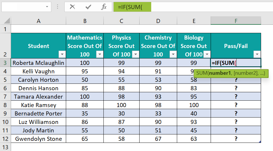
Next, as we require the aggregate secured by the student in each row, select the cell range B3:E3 to provide as the SUM() input.
=IF(SUM(Subject_Scores[@[Mathematics Score Out Of 100]:[Biology Score Out Of 100]]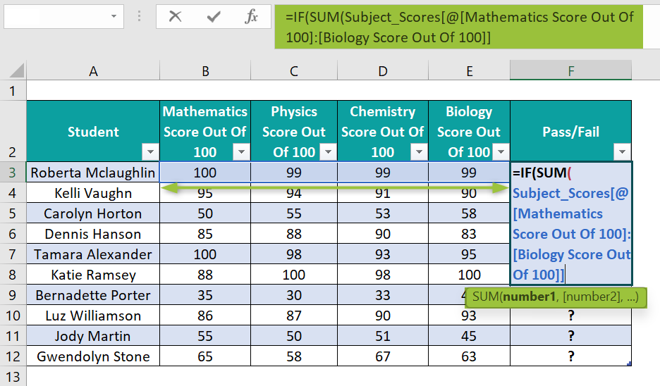
The above-mentioned selection creates Structured References to the chosen cell range.
Next, enter the closing bracket and complete the IF() formula, as shown below.
=IF(SUM(Subject_Scores[@[Mathematics Score Out Of 100]:[Biology Score Out Of 100]])>=250,”Pass”,”Fail”)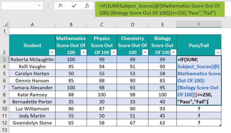
• Step 4: Press Enter to view the pass status in the target cell F3, and click the AutoCorrect Options button to update the formula in the remaining target cells F4:F12 automatically.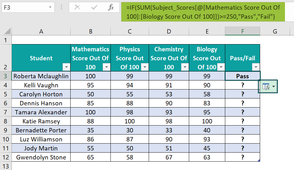
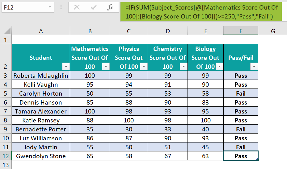
The SUM() finds the aggregate of marks, and the IF() checks if the determined aggregate of a student equals or is above the cutoff of 250. And if the condition holds in the target cell, the IF() returns the TRUE value, Pass. Otherwise, the IF() output is the FALSE value, Fail.
We cannot use Excel Structured References in conditional formatting.
The Excel Structured References may not work due to the following reasons:
• We would have copied and pasted the formula containing Structured References from a cell to the adjacent cells in the same row.
• We have used relative Structured References in place of absolute Structured References.
Use this Structured References In Excel Template to follow along with the examples in this article.
Download Excel Template