
What Is TRIM In Google Sheets?
TRIM in Google sheets, as the name suggests, helps users trim the data by removing the extra, multiple spaces. The function is available in both Excel and Google sheets.
Remember, we can trim, or in other words, eliminate the spaces in between each word. For example, consider the below table showing the name of a movie character, “Harry Potter” in column A.
Use this TRIM In Google Sheets Template to follow along with the examples in this article.
Download Excel Template
To begin with, select the cell B2 and enter the TRIM function formula, =TRIM(A2) and press Enter key. We will be able to find the result in cell B2, as shown in the below image.

In this article, let us learn how to trim our data using TRIM function with detailed examples.
Key Takeaways
- TRIM function in Google sheets helps users trim the data if there are extra spaces in the data.
- The syntax of TRIM function formula in Google sheets is TRIM(text) where text is the only mandatory argument.
- The text argument shows the string or reference which we want to trim in Google sheets.
- Remember, we can use SPLIT function and ARRAYFORMULA to split and trim content from one cell into multiple cells.
- We need to note that the arguments have correct number of arguments with parenthesis to avoid errors in Google sheets.
Syntax

The formula or syntax of TRIM in Google sheets is =TRIM(text)
where,
- text is the only mandatory argument showing the string or reference which we want to trim
How To Use TRIM In Google Sheets?
We can use TRIM function formula in two methods. They are:
- Select the TRIM Google sheets function under the Insert tab
- Manually enter the TRIM function
Method #1 – Select the TRIM Google Sheets function under the Insert tab
We can select the TRIM function via Insert tab using the below steps. They are:
Step 1: To begin with, we need to enter the data in the spreadsheets. Next, select the cell where we want to find the result.
Step 2: Next, select the Insert tab and click on the Text function category. Next, scroll down and click on the TRIM function.

Step 3: We will be able to see the TRIM function in Google sheets. Select the required arguments and press the Enter key.
We will be able to see the result in the active cell in Google sheets.
Likewise, we can use the TRIM function under the Insert tab.
Method #2 – Manually enter the TRIM function
We can manually enter the TRIM function using the below steps. They are:
Step 1: To begin with, we need to enter the data in the spreadsheets. Next, select the cell where we want to find the result.
Step 2: Next, enter =TR and select the TRIM function.

Alternatively, we can directly enter the TRIM function in Google sheets.
Step 3: We will be able to see the TRIM function. Select the required arguments and press the Enter key.
We will be able to see the result in the active cell in Google sheets.
Likewise, we can manually enter the TRIM function in Google sheets.
Examples
Now, let us learn how to use the TRIM function with the detailed following examples.
Example #1 – Basic Example
For example, consider the below table showing the proverb in column A and result in column B, respectively.

Now, let us learn how to use the TRIM function.
The steps are:
Step 1: To begin with, we need to enter the data in the spreadsheets. In this example, the data is available in the cell range A1:B4. Next, we need to select the cell where we want to find the result. In this example, we need to select the cell B2.
Step 2: Next, enter the TRIM function.
So, the complete formula is =TRIM(A2)

Step 3: Press Enter key.
We will be able to see the result in the cell B2, as shown in the below image.
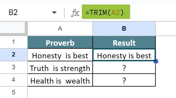
Now, using the AutoFill option, we can find the result in the cell range B3:B4, as shown in the below image.

Likewise, we can use the TRIM function.
Example #2 – Trim Whitespaces
For example, consider the below table showing the proverb in column A and result in column B, respectively.

Now, let us learn how to use the TRIM function.
The steps are:
Step 1: To begin with, we need to enter the data in the spreadsheets. In this example, the data is available in the cell range A1:B4. Next, we need to select the cell where we want to find the result. In this example, we need to select the cell B2.
Step 2: Next, enter the TRIM function in Google sheets.
So, the complete formula is =TRIM(A2)

Step 3: Press Enter key.
We will be able to see the result in the cell B2, as shown in the below image.

Now, using the AutoFill option, we can find the result in the cell range B3:B4, as shown in the below image.

Likewise, we can use the TRIM function.
Example #3 – Nested TRIM Function In Google Sheets
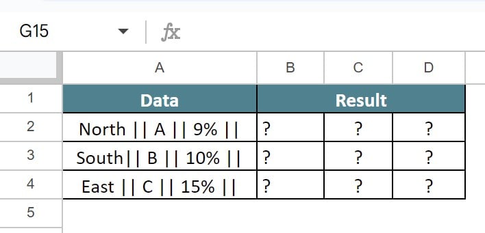
For example, consider the below table showing the data in column A, respectively.

Now, let us learn how to use the TRIM function.
The steps are:
Step 1: To begin with, we need to enter the data in the spreadsheets. In this example, the data is available in the cell range A1:D4. Next, we need to select the cell where we want to find the result. In this example, we need to select the cell B2.
Step 2: Next, enter the ARRAYFORMULA function.
So, the complete formula is =ARRAYFORMULA(TRIM(SPLIT(A2,”||”)))

Step 3: Press Enter key.
We will be able to see the result in the cell B2, as shown in the below image.

Now, using the AutoFill option, we can find the result in the cell range B3:B4, as shown in the below image.

Likewise, we can use the nested TRIM function.
Example #4 – TRIM With SPLIT Function
For example, consider the below table showing the proverb in column A and result in column B, respectively.
Now, let us learn how to use the TRIM function.
The steps are:
Step 1: To begin with, we need to enter the data in the spreadsheets. In this example, the data is available in the cell range A1:B4. Next, we need to select the cell where we want to find the result. In this example, we need to select the cell B2.
Step 2: Next, enter the TRIM function.
So, the complete formula is =ARRAYFORMULA(TRIM(SPLIT(A2,”||”)))

Step 3: Press Enter key.
We will be able to see the result in the cell B2, as shown in the below image.

Now, using the AutoFill option, we can find the result in the cell range B3:B4, as shown in the below image.

Likewise, we can use the TRIM function.
Important Things To Note
- TRIM function in Google sheets helps users trim the content by deleting the spaces.
- We need to make sure the data is selected in the argument is correct to avoid errors.
- Remember, we can use the IF function or other functions as nested functions in Google sheets.
Frequently Asked Questions (FAQs)
For example, consider the below table showing the proverb in column A and result in column B, respectively.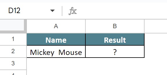
Now, let us learn how to use the TRIM function in Google sheets.
The steps are:
Step 1: To begin with, we need to enter the data in the spreadsheets. In this example, the data is available in the cell range A1:B2. Next, we need to select the cell where we want to find the result. In this example, we need to select the cell B2.
Step 2: Next, enter the TRIM function in Google sheets.
So, the complete formula is =TRIM(A2)
Step 3: Press Enter key.
We will be able to see the result in the cell B2, as shown in the below image.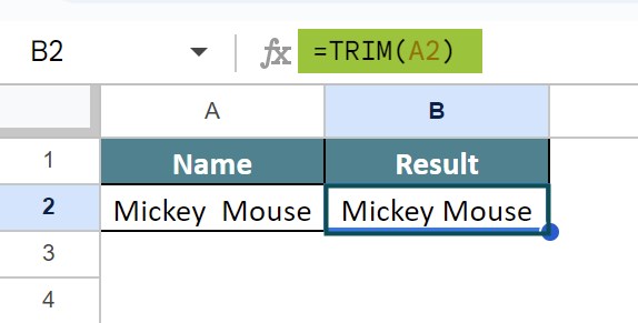
Likewise, we can use the TRIM function in Google sheets.
The difference between the SPLIT function in Google sheets and TRIM function is that,
• SPLIT function splits the data whereas, the TRIM function trims the content by eliminating the spaces.
TRIM function may not work if the data used in the formula does not match with the arguments. Similarly, the function wont work if the nested content in the formula does not have enough parenthesis.
Use this TRIM In Google Sheets Template to follow along with the examples in this article.
Download Excel Template