
What Is WORKDAY Google Sheets Function?
WORKDAY function in Google sheets is an inbuilt function used to find the end date or the last date after the mentioned number of days. This function is available in both Excel and Google sheets. Users can find the last day after the given number of days in the data. To use this function, we need to have the start date and the number of days included in the time period.
For example, consider the below table showing start date, and number of days in columns A and B, respectively.
Use this WORKDAY Google Sheets Function Template to follow along with the examples in this article.
Download Excel Template
Now, let us use the WORKDAY function in Google sheets with the help of the following steps. To begin with, select the cell C2 and insert the WORKDAY function in Google sheets formula, =WORKDAY(A2,B2). Now, press Enter key. We will be able to see the result in cell C2, as shown in the below image.

In this article, let us learn how to use WORKDAY function in Google sheets with detailed examples.
Key Takeaways
- WORKDAY function in Google sheets, as the name suggests, is a default function used to find the date after the given number of days.
- The function requires the start date and the number of days in the data.
- WORKDAY function formula in Google sheets is =WORKDAY(start_date,num_days,[holidays]) where start_date and num_days are the two mandatory arguments.
- The WORKDAY Google sheets function does not read non-numeric values and reads only numeric values in the format MM/DD/YYYY.
- Remember, to insert the formula properly in the arguments to avoid errors such as #VALUE! Error.
WORKDAY() Google Sheets Formula

The formula or syntax of WORKDAY function in Google sheets is =WORKDAY(start_date,num_days,[holidays])
where,
- start date is the starting date of the given period
- num_days is the number of days which we want to include and count the data
- holidays is the optional argument which shows the range or array with dates.
How To Use WORKDAY Google Sheets Function?
We can use WORKDAY Google sheets function in two different ways.
They are:
- Inserting the formula from the tab
- Manually entering the function
Method #1 – Inserting The Formula from The Tab
Step 1: To begin with, we need to open the Google sheets spreadsheet and insert the data.
Step 2: Next, select the cell where we want to find the result. Click on Insert tab.
Step 3: Next, select Function option. Click on Date in the drop-down options.
Step 4: Scroll down. Click on the WORKDAY option.
We will be able to see the function in the cell. Now, we can insert the cell range and find the end date using WORKDAY function in Google sheets.
Method #2 – Manually Entering The Function
Step 1: To begin with, we need to open the Google sheets spreadsheet. Insert the data.
Step 2: Next, select the cell where we want to find the result. Type =WORKDAY( and select the arguments.
Step 3: Alternatively, we can also type =W. Select WORKDAY function from the suggestions shown in Google sheets function.
Likewise, we can insert WORKDAY function in Google sheets.
Examples
Let us learn how to use WORKDAY function in Google sheets with detailed examples
Example #1
For example, consider the below table showing name of employees along with the start date, and number of days in columns A, B and C, respectively.

Now, let us use the WORKDAY function in Google sheets with the help of the following steps.
The steps are:
Step 1: To begin with, we need to insert the data in the spreadsheet. In this example, the data is available in the cell range A1:D10. Next, select the cell where we want to find the result. In this example, we need to select the cell D2.
Step 2: Next, insert the WORKDAY function formula.
So, the complete formula is =WORKDAY(B2,C2)
Step 3: Now, press Enter key.
We will be able to see the result in cell D2, as shown in the below image.

Now, using AutoFill option, we will be able to see the result in the cell range D3:D10, as shown in the below image.

Likewise, we can find the result, i.e., the last date or the end date in the given period.
Example #2
For example, consider the below table showing region (location) of organizations along with the start date, and number of days in columns A, B and C, respectively.

Now, let us use the WORKDAY function with the help of the following steps.
The steps are:
Step 1: To begin with, we need to insert the data in the spreadsheet. In this example, the data is available in the cell range A1:D5. Next, select the cell where we want to find the result. In this example, we need to select the cell D2.
Step 2: Next, insert the WORKDAY function formula.
So, the complete formula is =WORKDAY(B2,C2)
Step 3: Now, press Enter key.
We will be able to see the result in cell D2, as shown in the below image.

Now, using AutoFill option, we will be able to see the result in the cell range D3:D5, as shown in the below image.

Likewise, we can find the result, i.e., the last date or the end date in the given period.
Example #3
For example, consider the below table showing name of employees along with the start date, and number of days in columns A, B and C, respectively.

Now, let us use the WORKDAY function with the help of the following steps.
The steps are:
Step 1: To begin with, we need to insert the data in the spreadsheet. In this example, the data is available in the cell range A1:D5. Next, select the cell where we want to find the result. In this example, we need to select the cell D2.
Step 2: Next, insert the WORKDAY function formula.
So, the complete formula is =WORKDAY(B2,C2)
Step 3: Now, press Enter key.
We will be able to see the result in cell D2, as shown in the below image.

Now, using AutoFill option, we will be able to see the result in the cell range D3:D5, as shown in the below image.

Likewise, we can find the result, i.e., the last date or the end date in the given period.
Difference Between The WORKDAY And NETWORKDAYS Function In Google Sheets
The difference between the WORKDAY function and NETWORKDAYS function are:
- WORKDAY function gives us the last date (end date) of the given number of days.
- NETWORKDAYS function in Google sheets gives the number of working days with respect to the starting and ending date of the given period.
Important Things To Note
- WORKDAY function finds the date after the given number of days.
- In other words, the function finds the end date or last date from the given period.
- The function is categorized under Insert tab, grouped under Functions category, found under Date sub-group.
- Usually, WORKDAY function is confused with NETWORKDAYS function but remember that the WORKDAY function gives us the end date or last date from the given data.
- Whereas, the NETWORKDAYS function shows us the total number of work days, including the start date and end date.
Frequently Asked Questions (FAQs)
For example, consider the below table showing name of employees along with the start date, and number of days in columns A, B and C, respectively.
Now, let us use the WORKDAY function with the help of the following steps.
The steps are:
Step 1: To begin with, we need to insert the data in the spreadsheet. In this example, the data is available in the cell range A1:C2. Next, select the cell where we want to find the result. In this example, we need to select the cell C2.
Step 2: Next, insert the WORKDAY function formula.
So, the complete formula is =WORKDAY(A2,B2)
Step 3: Now, press Enter key.
We will be able to see the result in cell C2, as shown in the below image.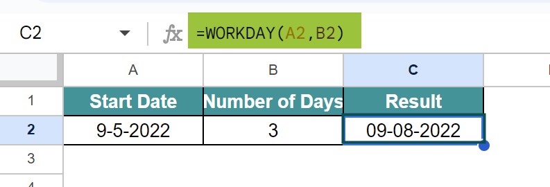
Likewise, we can find the result, i.e., the last date or the end date in the given period.
The formula or syntax of NETWORKDAYS function in Google sheets is =NETWORKDAYS(start_date,end_date,[holidays])
where
start date is the starting date of the given period
end date is the last date of the given period
holidays is the optional argument which shows the range or array with dates.
Remember, WORKDAY function in Google sheets may not work when
• The data we have has date in non-numeric version. In other words, we should not have any text characters.
• For example, the WORKDAY function does not read 31st January 2020 format. Instead, the function reads only 31/1/2020.
Use this WORKDAY Google Sheets Function Template to follow along with the examples in this article.
Download Excel Template