
What Is Covariance Matrix on Excel?
The covariance matrix on Excel is a square matrix that contains the covariance between different variables. It helps evaluate the structured relationships among the variables in a given dataset.
Users can use the Excel covariance matrix in financial engineering, machine learning, and econometrics for applications such as principal component analysis.
Use this Covariance Matrix on Excel Template to follow along with the examples in this article.
Download Excel TemplateFor example, the below table contains the per-day stock prices of top tech US companies.
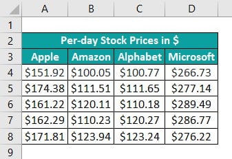
Suppose the requirement is to assess the relationships between the specified companies based on their per-day stock prices. Then, we can calculate covariance matrix in Excel for the above data using the Data Analysis ToolPak feature from the Data tab and perform the required analysis.
And interpreting covariance matrix in Excel is quite straightforward.
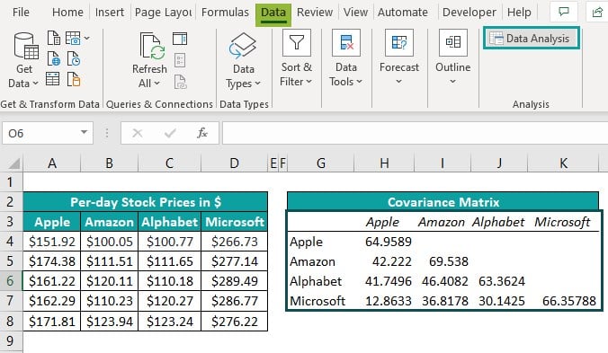
For example, in the above scenario, the variances of Apple, Amazon, Alphabet, and Microsoft per-day stock prices are 64.9589, 69.53802, 63.36238, and 66.35788.
On the other hand, the covariance between:
- Apple and Amazon per-day stock prices- 42.22199
- Apple and Alphabet per-day stock prices- 41.74961
- Apple and Microsoft per-day stock prices- 12.86334
- Amazon and Alphabet per-day stock prices- 46.4082
- Amazon and Microsoft per-day stock prices- 36.81778
- Alphabet and Microsoft per-day stock prices- 30.14246
Further, as all the matrix values are positive, the inference is that the specified companies’ per-day stock prices increase or decrease in tandem.
Key Takeaways
- The covariance matrix on Excel is a square matrix, which is symmetrical along its diagonal. It helps determine whether two variables vary linearly in the same direction or inversely. And while its diagonal shows the variances of the variables, the part below the diagonal contains the covariances between the variables.
- Users can use the covariance matrix in applications such as performing Cholesky decomposition in Stochastic Modelling.
- We can create a covariance matrix using the Data Analysis ToolPak feature in the Data tab.
Explanation And Uses
Covariance statistically indicates whether variables vary in tandem or inversely with each other. And the formula to calculate covariance matrix on Excel is:
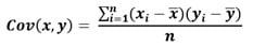
The covariance matrix values lie between (-∞,∞). And they are unit dependent, with their signs deciding whether two variables vary directly or inversely.
If the matrix value is positive, the two variables increase and decrease in the same direction. And a negative value implies that if one variable increases, the other decreases.
Thus, we can use the above expression as a covariance matrix Excel formula and create square covariance matrices, depending on the number of variables involved. For instance, if the source data includes two variables, we can build a 2×2 matrix. And for a three variables dataset, we can find a 3×3 covariance matrix.
Furthermore, the resulting matrix will be symmetrical towards the diagonal. In other words, the part above the diagonal is a mirror image of the part below the diagonal containing the covariance values. And so the output matrix has the section above the diagonal empty.
The covariance matrix uses are:
- Review the dependency behavior between two vectors in machine learning.
- Correlate variables while performing Stochastic Modeling in financial engineering.
- Determine the eigenvectors during principal component analysis.
- Estimate the returns on financial assets.
How To Use Covariance Matrix In Excel?
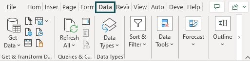
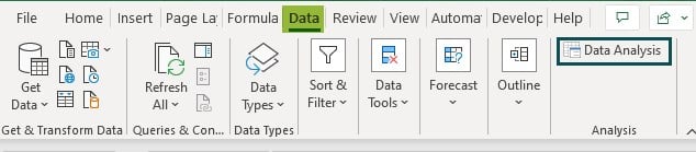
We can use the covariance matrix from Data Analysis ToolPak in the Data tab in Excel.
Click on a cell in the active worksheet and select the Data tab – click Data Analysis.
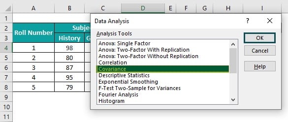
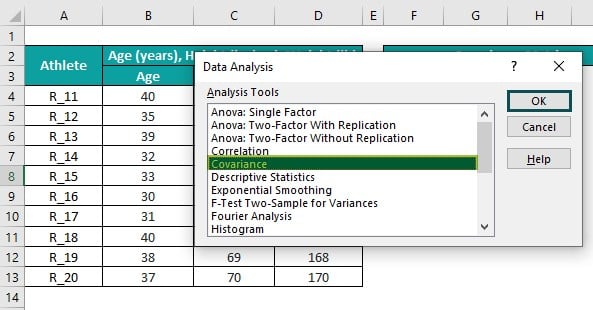
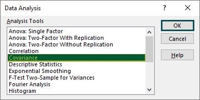
The Data Analysis window will open, where we must select Covariance from the Analysis Tools list and click OK.
The Covariance window will open. Update the highlighted fields and click OK to obtain the required square covariance matrix in the active worksheet.
But before we see an example of calculating the covariance matrix with the Data Analysis ToolPak, we must confirm that the Data Analysis feature is available in the Data tab.
And suppose the Data Analysis feature is not available in the Data tab (as shown below).
Then the steps to install it are as follows:
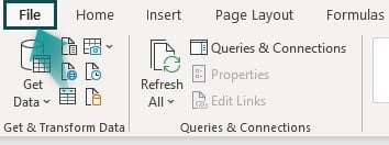
Step 1: First, click File tab – Options to open the Excel Options window.

Step 2: Next, select the Excel Add-ins category in the Excel Options window and then, click Go.
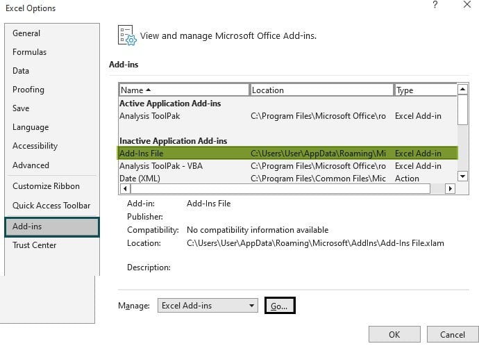
The Add-ins window will open.
Step 3: Then, check the Analysis ToolPak option from the Add-ins list in the Add-ins window.
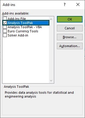
And once we click OK in the Add-ins window, the Data Analysis feature will be visible in the Data tab.
#Basic Example
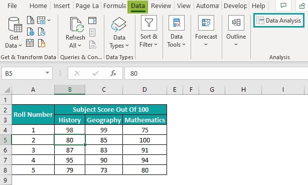
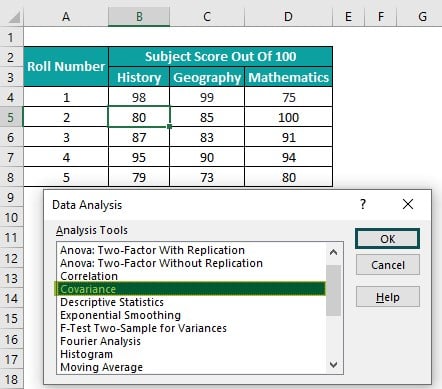
The following table contains scores secured by five students in three subjects.
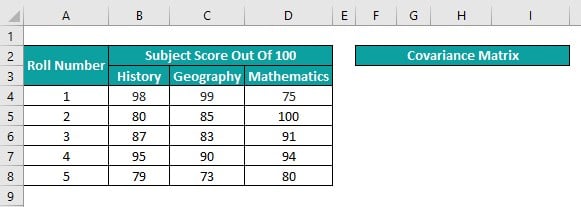
Suppose the requirement is to perform the covariance analysis in excel based on the scores each student secured in the three subjects. Then, we can create a covariance matrix in the current sheet for the above data to perform the required analysis.
Step 1: Click on a cell in the active worksheet and follow the path Data – Data Analysis to open the Data Analysis window.

Step 2: Pick Covariance from the Analysis Tools list and click OK to close the Data Analysis window.
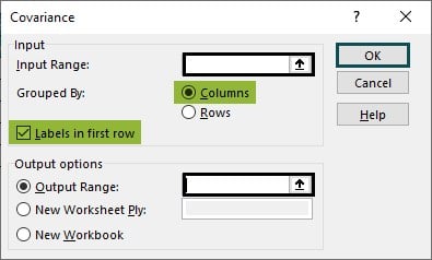
Step 3: The Covariance window opens, where we need to update the fields as depicted below.
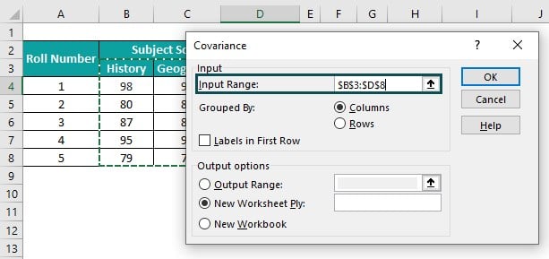
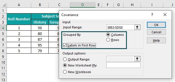
When selecting the Input range, include the cells containing the subject names in the selection. And check the Labels option in the Covariance window to view the subject names in the resulting covariance matrix.
Also, grouping is by column in the source data. So, the Grouped By option is Columns.
And as we require the covariance matrix in the current worksheet, pick the first option under Output options and enter the reference to the required target cell.
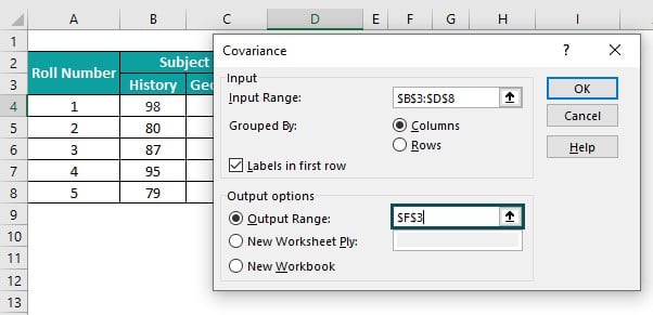
Click OK. It will close the Covariance window, and we will obtain the following covariance matrix.
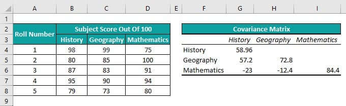
Thus, we can obtain a square matrix with the part above the diagonal empty, as the covariance matrix is symmetric along the diagonal.
We shall first list the variances and covariances required for interpreting covariance matrix in Excel.
The variances of the subjects’ scores are on the matrix diagonal:
- History score: 58.96
- Geography score: 72.8
- Mathematics score: 84.4
The covariances between the specified subjects are in the section below the diagonal:
- History and Geography scores: 57.2
- History and Mathematics scores: -23
- Geography and Mathematics scores: -12.4
The above covariance matrix shows positive covariance between History and Geography. It implies that students who score high in History also score well in Geography. And those who score low in History also score low in Geography.
On the other hand, the covariances between History and Mathematics and Geography and Mathematics are negative. The two negative values imply that those who score well in History and Geography perform poorly in Mathematics. Likewise, those who score well in Mathematics perform poorly in History and Geography.
Examples
Check out the following Excel covariance matrix examples to use the matrix in the best ways possible.
Example #1
The table below shows a list of athletes, their ages, heights, and weights.

Suppose the requirement is to perform the covariance analysis of the athletes’ statistics. Then, calculating the covariance matrix in the current worksheet based on the above data is the best solution.
Step 1: Click on a cell in the current worksheet and follow the path Data – Data Analysis to open the Data Analysis window.

Step 2: Pick Covariance in the Data Analysis window, and click OK to open the Covariance window.
Step 3: Update the highlighted fields in the Covariance window.
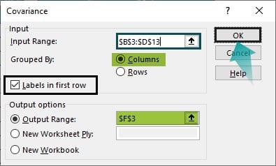
The input range includes the Age, Height, and Weight columns, starting from the column headers in the cell range B3:D3. And we must check the labels option to include them in the matrix.
On the other hand, grouping is by column in the source data. So, the Grouped By option is Columns.
And as we require the covariance matrix in the active worksheet, we select the first option under Output options and provide the target cell reference in excel.
Step 4: Click OK in the Covariance window to view the required covariance matrix.

Thus, the above covariance matrix shows that the athletes’ Age, Height, and Weight variances are 13.05, 21.65, and 17.85. And the covariances between Age and Height, Age and Weight, and Height and Weight are 7.95, 7.85, and 19.05.
Furthermore, the covariance values in the section below the diagonal are positive. So, the inference is that the Age and Height, Age and Weight, and Height and Weight vary linearly in the same direction.
Example #2
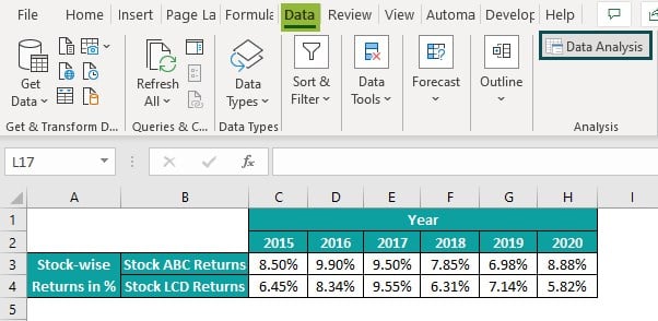
The following table shows the percentage returns from two stocks, ABC and LCD, during 2015-20.

Suppose the requirement is to determine the polarity of the linear relationship between the stocks based on the yearly returns.
Then, we can create a covariance matrix for the above dataset, where the data grouping is by rows.
Step 1: Click on a cell in the active worksheet and follow the path Data – Data Analysis to open the Data Analysis window.
Step 2: In the Data Analysis window, pick the Covariance analysis tool, and click OK.
Step 3: The Covariance window will open. Here, we need to update the below-highlighted fields.
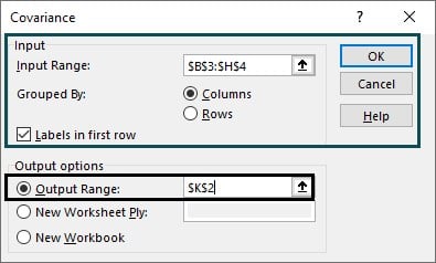
The input range includes the yearly returns from each stock and the stock names. And we check the labels option to view the stock names in the resulting matrix.
However, as the grouping is by rows in the source data, the Grouped By option should be Rows.
And we provide the target cell reference K2 to view the covariance matrix in the current sheet.
Step 4: Click OK in the Covariance window to close it and obtain the following covariance matrix.
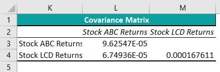
The stock ABC and LCD returns’ variances are on the matrix diagonal, 0.0000962547 and 0.000167611, respectively. And the covariance between stock ABC and LCD returns 0.0000674936111111111.
Further, as the covariance between the two stocks’ returns is positive, they vary linearly in random or in the same direction.
Example #3
The below image shows two tables.
The first table contains three variables’ datasets, X, Y, and Z.
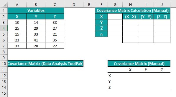
Suppose the requirement is to create a covariance matrix for analyzing the relationships between the specified variables in Excel.
Then, here is how we can use the Data Analysis ToolPak and achieve the matrix in the target cell A11.
Also, we shall use the second table and covariance matrix excel formula to calculate the covariance matrix manually and display the result in cell G11. The variable n has the value 5 assigned as it denotes the total number of data points in each data series.
Step 1: Click on a cell in the active worksheet and choose Data – Data Analysis to open the Data Analysis window.

Step 2: Pick Covariance from the Analysis Tools list in the Data Analysis window and click OK.
The Covariance window opens, where we must update the highlighted fields and then, click OK.

The input range is A2:C7, which includes the three variables’ datasets and the variable names. And the grouping is by Columns, with the labels option enabled to view the variable names in the resulting covariance matrix.
Also, the target cell is A11. So, it is the output range.
Clicking OK in the Covariance window will result in the below-highlighted covariance matrix.

We shall now see the manual covariance matrix calculations.
Step 3: Select cell G2, enter the AVERAGE excel function to obtain the mean value of variable X and press Enter.
=AVERAGE(A3:A7)

Next, select cell G3, enter the AVERAGE()to obtain the mean value of variable Y and press Enter.
=AVERAGE(B3:B7)

Select cell G4, enter the AVERAGE()to obtain the mean value of variable Z and press Enter.
=AVERAGE(C3:C7)

Next, we must find the difference between each data point in a dataset and the dataset mean value for the three variables.
Step 4: Select cell H3, enter the below formula, and press Enter.
=A3-$G$2

Using the fill handle in excel, enter the formula in cell range H4:H7.

Step 5: Select cell I3, enter the below formula, and press Enter.
=B3-$G$3

Using the fill handle, enter the formula in cell range I4:I7.

Step 6: Select cell J3, enter the below formula, and press Enter.
=C3-$G$4

Using the fill handle, implement the formula in cell range J4:J7.

Step 7: Select cells from H12 to J14, one at a time. And enter the expression specified in the Formula Bar to determine the corresponding covariance matrix elements using the covariance matrix formula.


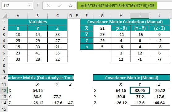


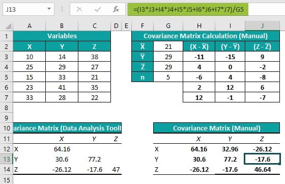

Thus, the output shows that the two methods result in the same covariance matrix.
Further, the manual method proves that the covariance matrix is symmetric along the diagonal.
For example, cells H13 and I12 show the covariance between X and Y. And both the cells contain the same value, 30.6.
And, as the covariance between X and Y is positive, the two variables vary linearly in the same direction. On the other hand, the covariances between X and Z and Y and Z are negative, implying the variable pairs X and Z and Y and Z vary inversely.
Important Things To Note
- Ensure the data series do not have non-numeric values. Otherwise, we will get a warning message, and we cannot create a covariance matrix in Excel.
- Suppose we calculate a covariance matrix. Then, any changes made to the source data will not update the matrix automatically. Also, clicking Ctrl + Z will not undo the covariance matrix calculations. For any changes in the matrix, we must delete the existing one and repeat the steps to create a new matrix.
- The covariance matrix obtained using the Data Analysis ToolPak contains population variances in its diagonal, not the sample variances.
Frequently Asked Questions (FAQs)
We can calculate the variance-covariance matrix in Excel in the following way. Let us see the steps with an example.
The table below contains the expected daily returns of three firms.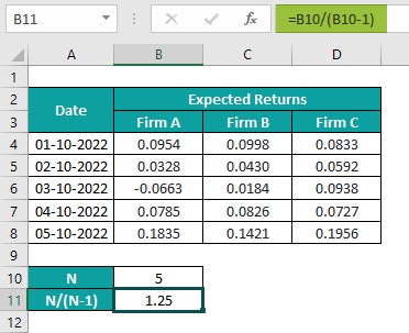
Suppose the total number of data points in each firm’s data series is 5.
And the requirement is to determine the sample variance-covariance matrix for the above data. Then, we can create a covariance matrix using the Data Analysis ToolPak feature in the Data tab. And then, we can derive the sample variance-covariance matrix using the calculated matrix and the highlighted cell B11 formula.
Step 1: Click a cell in the active worksheet and choose Data – Data Analysis to open the Data Analysis window.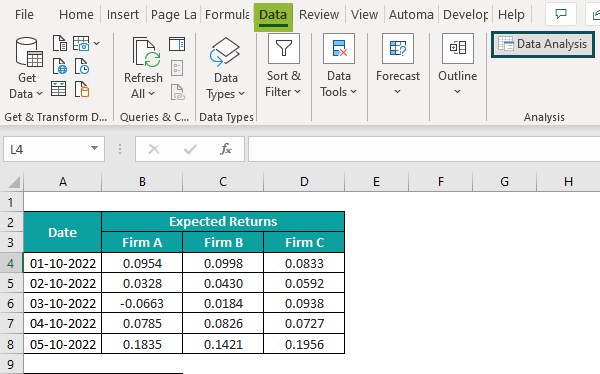
Pick Covariance from the Analysis Tools list in the Data Analysis window. And click OK.
The Covariance window will open, where we must update the highlighted fields, as shown below.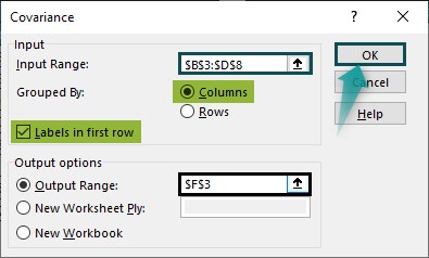
Click OK to close the Covariance window and view the covariance matrix in the specified target cell.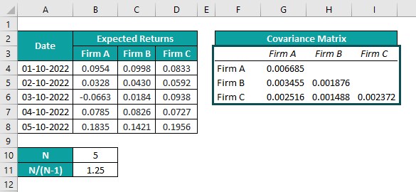
The following steps will complete the matrix as it is symmetric along the diagonal.
Step 2: Select cell range G5:G6, press Ctrl + C to copy the values, and click cell H4. And then, press Alt + E + S to open the Paste Special Window and check the Transpose option. Click OK to execute the action.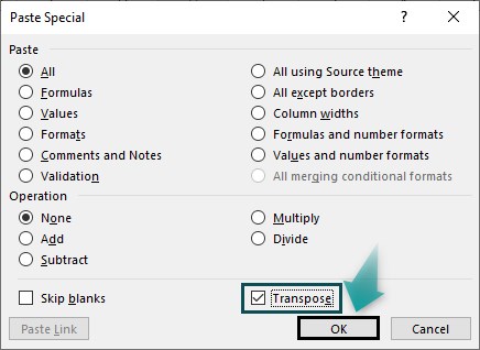
Then two values will get pasted row-wise in cell range H4:I4.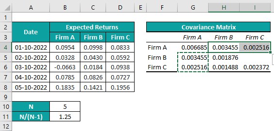
Next, select cell H6, press Ctrl + C to copy the cell value, and click cell I5. And press Ctrl + V to paste the value in cell I5.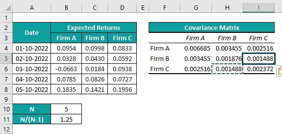
The calculated covariance matrix contains the population variances of the three firms’ daily expected returns in the diagonal.
But, assuming the given data set is massive. Then, ideally, we must calculate the sample variance instead of the population variance. So, in the above scenario, we can modify the covariance matrix to obtain a matrix with sample variances of the three firms’ daily expected returns in its diagonal.
Step 3: Select the cell range G11:I13 and enter the below formula.
=B11*G4:I6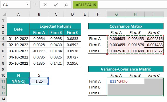
And press Ctrl + Shift + Enter to apply the above expression as an array formula to achieve the required variance-covariance matrix.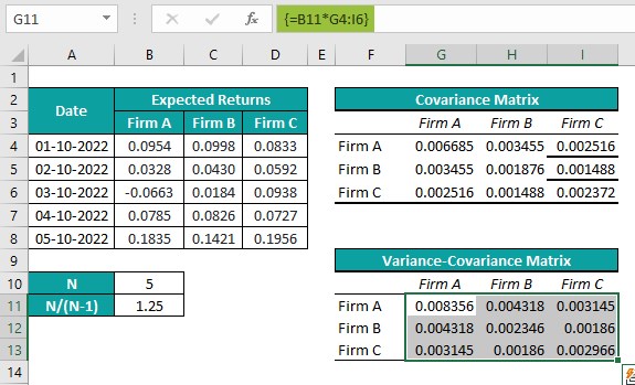
Cells G11, H12, and I13 show the sample variances of each firm’s daily expected returns. And we can verify the values using the VAR.S().
We shall introduce a new table below the variance-covariance matrix to show the sample variances of the three firms’ daily expected returns using the VAR.S().
Step 4: Select cell G16, enter VAR.S(), and press Enter.
=VAR.S(B4:B8)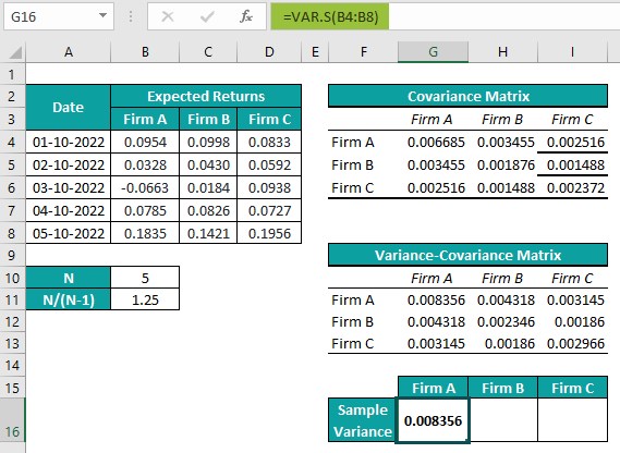
Select cell H16, enter VAR.S(), and press Enter.
=VAR.S(C4:C8)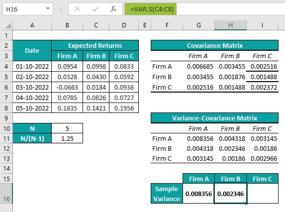
Select cell I16, enter VAR.S(), and press Enter.
=VAR.S(D4:D8)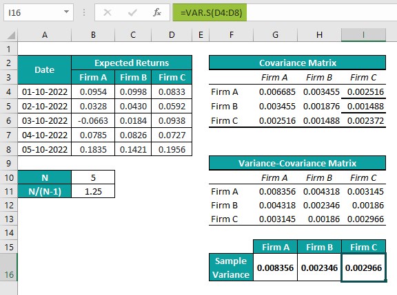
Thus, we see that the sample variances in the variance-covariance matrix and the VAR.S() outputs in the sample variance table are the same for each firm’s daily expected returns.
The use of covariance matrix in Excel is that it helps understand the relationships in a matrix of specified variables. We can use it to decorrelate the given variables or transform them into other variables.
The covariance matrix in Excel is not working because the source data contains non-numeric values or invalid numbers.
Use this Covariance Matrix on Excel Template to follow along with the examples in this article.
Download Excel Template