
What is FLATTEN in Google Sheets?
FLATTEN in Google Sheets converts a range or array into a single column. It takes multiple rows and columns and stacks them vertically into a single column. This function is very helpful when one has data spread across rows and columns, but one wished the data to be in a single list for certain purposes and calculations. It is used in scenarios such as filtering duplicates or to run a function that only works on one-dimensional arrays. FLATTEN helps simplify your dataset and offers it more flexibility across various functions.
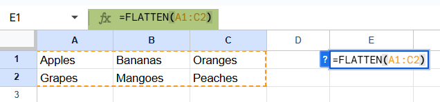
For example, we have some values in the cells A1:C2. We apply the function as shown below: =FLATTEN(A1:C3).
Use this FLATTEN in Google Sheets Template to follow along with the examples in this article.
Download Excel TemplateThe result of this formula is as shown in the screenshot below. This change after applying the function makes it easier to combine it with other functions like UNIQUE to the data set without worrying about its original layout.

Key Takeaways
- The FLATTEN function in Google Sheets transforms a multi-row and multi-column range into a single vertical column of values.
- Its syntax is as follows: =FLATTEN(range). Here, range refers to the group of cells you want to combine into a single column.
- The function processes the data left to right, top to bottom, maintaining the original order of values in the source range.
- FLATTEN in Google Sheets is powerful when combined with other functions like UNIQUE, SORT, or FILTER to clean and organize large and complex datasets.
- Empty cells will be included in the output as blank entries.
Syntax
Before proceeding further, let us look at the FLATTEN formula in Google Sheets. The syntax of the FLATTEN function is as follows:
=FLATTEN(range)
Arguments:
“range” – the array or range of values that you wish to convert into a single column.
It can be anything from a mix of rows and columns, or even multiple arrays combined.
The FLATTEN function processes the values in the range from left to right and top to bottom. It then stacks them into a single vertical list. It ignores empty cells and maintains the order in which the values appear in the original range.
How To Use FLATTEN Function in Google Sheets?
FLATTEN in Google Sheets helps convert a range of values into a single column, making it easier to work with scattered or multi-dimensional data. This is particularly helpful when you want to simplify a dataset for functions like UNIQUE, SORT, or FILTER.
You can use the FLATTEN function in two main ways:
- By manually typing FLATTEN in Google Sheets
- By selecting it from the Google Sheets menu
Using the FLATTEN Function Manually
Let’s go through an example to understand how to use FLATTEN step-by-step when entering the formula manually.
Let us suppose we have some fruits’ values in a range, as shown below. All these fruits should be listed in a single vertical column.
Step 1: Enter the data into cells A1 to C2 in a sheet. Each cell should contain a different fruit name, as shown above.

Step 2: Choose an empty cell (here we choose E1) where you want the output of the FLATTEN function to appear. Type the function name as shown with an open parentheses.
=FLATTEN(

Step 3: Inside the parentheses, specify the range of values you want to flatten. Here, we enter the range as:
=FLATTEN(A1:C2).
Step 4: Press Enter.
The function will automatically return a vertical list with all six fruit names stacked in a single column: Apples, Bananas, Oranges, Grapes, Mangoes, Peaches. This helps organize the data for analysis or filtering.

Using FLATTEN From the Menu
If you prefer to use the function from the built-in function menu:
- Go to Insert → Function → Lookup.
- Select FLATTEN from the dropdown list.
- Highlight the cell range (e.g., A1:C2) or type it into the formula bar.
- Press Enter to see the results in a single vertical list.
The FLATTEN function is especially helpful for cleaning up and reorganizing data that’s spread across rows and columns.
Examples
Let us look at different real-time scenarios where we can use the FLATTEN function in Google Sheets.
Example #1
A marketing team has a contact list of clients spread across multiple rows and columns. Each row contains client email addresses grouped by region. However, the team needs a single-column list of email addresses for a printout. To prepare the data, they must first convert the multi-row contact table into a single column. FLATTEN in Google Sheets can do this instantly.
Step 1: Open a new sheet and enter the data into a 3×3 table as shown below. You can also notice an empty cell.

Each cell contains a different email address from different teams.
Step 2: The team must choose an empty cell like E1 for the final list to appear. Now enter the following formula:
=FLATTEN(A1:C3)

Step 3: Press Enter. You get the email addresses in a single vertical column.

You can notice how the empty cell has been considered as it is. This technique saves time and avoids manual copy-pasting when dealing with multi-row or multi-column datasets. It is very useful whether you are emailing contacts, products, or survey responses. The function converts disorganized arrays into linear lists. This is useful for even exporting to external systems.
Example #2 – Using FLATTEN with UNIQUE Function
A person is analyzing data from a survey in a company where employees were allowed to select their favorite apps. Each department submitted its responses in a different column. However, many employees selected the same apps. Let us create a clean list of unique tools preferred across the company.
Let us use the FLATTEN in Google Sheets along with UNIQUE to instantly generate a de-duplicated list.
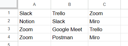
Step 1: Enter the following data into the sheet in a range.
Many of the tools are repeated.
Step 2: In cell E1, enter the following formula with the UNIQUE function:
=UNIQUE(FLATTEN(A1:C4))
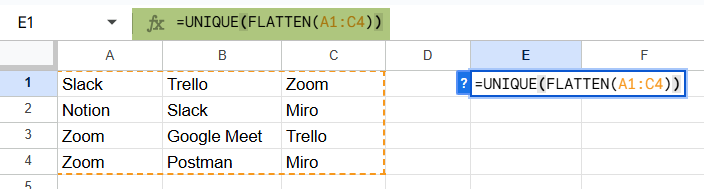
Step 3: Press Enter.
The formula first flattens the 4×3 range into a single column and then filters out duplicate entries. The output is as shown below:
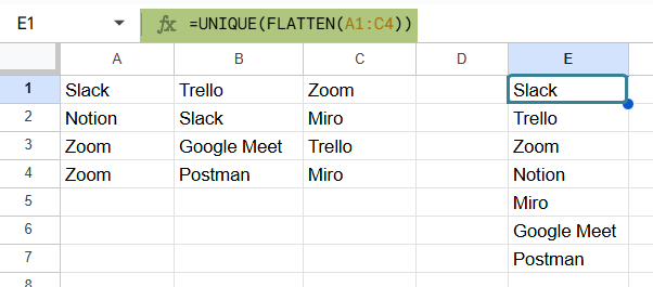
This combination of FLATTEN and UNIQUE is a powerful way to summarize the information. It’s useful in surveys or datasets where you want a quick, neat list of distinct values from a grid. It saves time and gives us an efficient list.
Example #3 – Using FLATTEN with Conditional Formatting
A teacher collects project topic preferences from different student groups. Each group lists its favorite topics in separate columns. However, the teacher wished to visually identify which project topics are the most popular across all groups. These have been selected more than once. The teacher uses FLATTEN with Conditional Formatting to highlight repeated topics instantly. Let us see how it is done.
Step 1: Enter the following data into cells A1:C4. Each row represents the student’s top three choices. Some values may be repeated.

Step 2: Select the full range A1:C5. Go to the menu:
Format → Conditional formatting
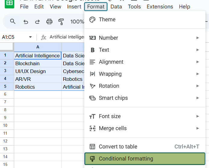
Step 3: In the pane on the right, under Format cells if, select Custom formula is, and enter the following formula:
=COUNTIF(FLATTEN($A$1:$C$4), A1) > 1
This formula checks if the value in each cell appears more than once in the flattened range.
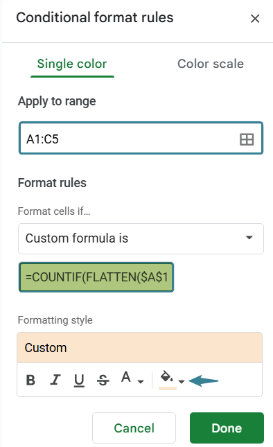
Step 4: Choose a highlight color and click Done. Observe the range for the unique values.

All the project topics that appear multiple times across the table will be highlighted automatically. This makes it easy to spot popular choices immediately.
Important Things to Note
- Empty cells within the range are included as blank entries in the output.
- FLATTEN works with arrays, ranges, and combinations of ranges, but it does not remove duplicates or sort the data by itself.
- Non-contiguous range rows are treated as continuous data when flattened.
- FLATTEN is especially useful when combined with other functions like UNIQUE or FILTER to further work on the output list.
- Since FLATTEN outputs a dynamic array, ensure there is enough space below the formula to avoid overwriting existing data.
Frequently Asked Questions (FAQs)
If a single multi-column range is provided, FLATTEN in Google Sheets will stack the values row by row. For example, in a single range, it will list A1, followed by B1, then C1. Next, A2, then B2, and so on. However, if columns are provided as separate ranges, they are stacked column by column.
FLATTEN is often used in conjunction with other functions like FILTER, UNIQUE, or SPLIT to perform complex data manipulations, such as filtering and flattening data, or splitting it based on a delimiter before flattening.
1. Creating a single master list from multiple smaller lists in different ranges.
2. Preparing data for analysis that requires a single-column input.
3. Consolidating survey responses into a single list.
4. Making a single list for exporting to external sources.
Use this FLATTEN in Google Sheets Template to follow along with the examples in this article.
Download Excel Template