
What Is Group In Google Sheets?
Group in Google Sheets is an option that enables us to group rows or columns, that we can collapse and expand according to our requirements. Our data appears brief as we can hide the grouped data. On the flip side, we can also show our data in detail, as we can unhide the grouped data.
Users can utilize the Group option in Google Sheets to arrange their massive dataset in a specific structure, which makes navigating and managing the data more straightforward. It also helps in enhancing data privacy and improves data readability and presentation.
Use this Group In Google Sheets Template to follow along with the examples in this article.
Download Excel TemplateFor instance, the following dataset contains the sales figures of six branch offices of a firm.

Consider that we must display only the total sales figures of all the branch offices while keeping the monthly sales figures hidden.
Then, adhering to the definition of Group in Google Sheets explained earlier, we can use the Group option to achieve the required outcome.

Let us see the steps to create group in Google Sheets, which will help us hide the monthly sales figures in the final dataset display.
First, click on the column B header to select the entire column. Next, while holding the Ctrl key, click on the columns C and D headers to select the complete columns. Next, select the Group in Google Sheets option right arrow under the View tab in the ribbon, after which we must choose the option Google Sheets Group columns B – D option, which is similar to Excel Group Columns option.
We will now see the three columns grouped, denoted by the expanded outline with the ‘–‘ button on the left end of the line and above column A.
Next, as we need to hide the grouped columns B-D, we can click the ‘–‘ button to collapse the group. This action will show the ‘+‘ button above column A, indicating that the three columns are hidden and we can only view the outline.
On the flip side, clicking the ‘+‘ button will expand the group, unhiding the grouped columns.
Key Takeaways
- The option Group in Google Sheets helps us group a set of continuous rows or columns, which we can collapse and expand to suit our needs. We can collapse grouped rows or columns to hide the specific rows or columns. In contrast, expanding the grouped rows or columns will unhide the concerned rows or columns.
- The keyboard shortcuts to group rows or columns in Google Sheets are Alt + Shift + 🡪 in Windows and Option + Shift + ► in Mac. However, before using the shortcut, please select the concerned rows or columns.
- The Group option in Google Sheets enables us to make the dataset more efficient for analysis. Also, the option helps make the dataset more presentable as we can hide irrelevant data and highlight only the key information in the given dataset.
How To Group Rows And Columns In Google Sheets?
We shall see the methods to group rows and columns using the Group function, in line with the definition of Group in Google Sheets explained previously.
Group Rows And Columns Using Menu
We can group rows and columns using the Group option in the menu, as described below:
Grouping Rows
The steps to create group in Google Sheets for a set of rows using the Group option in the menu are as explained below:
- Choose the rows that we aim to group. We must select the complete rows by first clicking the number of the first row on the leftmost end of the workspace in the set of rows we aim to group to select the entire row. Then, while pressing the Ctrl key, we must click the row numbers of the specific rows to select the required rows. For instance, say, we choose rows 2 and 3.

- Select the View tab – The Group option right arrow – The Group rows 2 – 3 option (the row numbers in this option will vary according to the rows we choose to group).

[Alternatively, we can choose the required continuous rows and then hover the mouse cursor over the chosen rows and right-click to access the popup menu.

Next, scroll down the popup menu to choose the View more row actions option right arrow. Next, select the Group rows 2 – 3 option, as shown above.]
The abovementioned steps will group the chosen rows, indicated by a gray vertical block on the left of the row numbers. The block contains a line starting with a ‘–‘ button on the left of one row above the first row in the grouped rows and ending at the last row in the grouped rows.

Please note that we cannot group non-contiguous rows, as in such a case the Group in Google Sheets option will appear disabled.
Grouping Columns
The steps for using Group in Google Sheets from the menu to group a set of columns are as described below:
- Please select the columns that we aim to group. We must select the complete columns by first clicking the letter of the first column at the top of the workspace in the set of columns we aim to group to choose the entire column. Then, while pressing the Ctrl key, we must click the column letters of the required columns to choose the specific columns. For example, say we select columns B and C.

- Choose the View tab – The Group option right arrow – The Group columns B – C option (the column letters in this option will vary with the columns we choose to group).

[Alternatively, we can select the required continuous columns and then hover the mouse cursor over the selected columns and right-click to view the popup menu.

Next, scroll down the popup menu to select the View more column actions option right arrow. Next, click on the Group columns B – D option, as depicted above.]
These steps will group the specific columns, indicated by a gray horizontal block above the column letters. The block shows a line starting with a ‘–‘ button above the column on the left of the first column in the grouped columns and ending at the last column in the grouped columns.

Please note that we cannot group non-contiguous columns, as in such a scenario the Group option will appear disabled in the menu.
Furthermore, we can also change the position of the +/– button, appearing after the grouping. For that, we must right-click the ‘+’ button or the ‘–’ button to open the popup menu. Next, choose the Move +/- button to the bottom option or the Move +/- button to the right option from the popup menu, depending on whether we have grouped rows or columns.


Group Rows And Columns Using Keyboard Shortcuts
We can group the chosen rows or columns using Group in Google Sheets keyboard shortcuts mentioned below:
- Windows: Alt + Shift + 🡪
- Mac: Option + Shift + ►
How To Collapse Rows And Columns In Google Sheets?
We can collapse rows and columns in Google Sheets by clicking on the corresponding ‘–’ button.
Otherwise, we can right-click the ‘–’ button to open the popup menu. Next, choose the Collapse row group option from the popup menu. It is to collapse the specific grouped rows and the Collapse column group option to collapse the specific grouped columns.
Considering the previous illustration, we must collapse the grouped rows 2 and 3. Also collapse grouped columns B and C in the following dataset.

We shall press the ‘–’ button on the left of the row numbers to collapse the grouped rows.
[Otherwise, right-click the ‘–’ button on the left of the row numbers to open the popup menu.

Next, choose the Collapse row group from the popup menu.]

Next, press the ‘–’ button on top of the column letters to collapse the grouped columns.
[Otherwise, right-click the ‘–’ button above the column letters to open the popup menu.

Next, choose the Collapse column group from the popup menu.]

Thus, we see the specific row and column groups collapsed.
How To Expand Rows And Columns In Group In Google Sheets?
We can expand rows and columns in Google Sheets by clicking on the corresponding ‘+‘ button.
Considering the previous example, we should expand the grouped rows 2 and 3 and the grouped columns B and C in the following dataset.

We shall press the ‘+’ button on the left of the row numbers to expand the grouped rows.

Next, press the ‘+’ button on top of the column letters to expand the grouped columns.

How To Ungroup Rows And Columns In Google Sheets?
We can ungroup rows and columns in Google Sheets as explained below:
- Right-click on the ‘+’ or ‘–’ button to open the popup menu. Next, select the Remove Group option from the popup menu.
Continuing with the previous example, consider that we must ungroup the grouped rows 2 and 3. Then, we shall right-click the ‘–’ button on the left of the row numbers to choose the Remove Group option from the popup menu.

The above action will ungroup the specific rows.

Next, consider that we should ungroup the grouped columns B and C. Then, we shall right-click the ‘–’ button on the top of the column letters to open the popup menu, where we choose the Remove Group option.

The above action will ungroup the specific columns.

However, assume the dataset is massive and contains multiple groups. Then, in such scenarios, the steps to ungroup rows or columns are the following:
- Click on the first row or column in the set of rows or columns we have grouped. Next, while pressing the Ctrl key, click on the remaining contiguous row numbers or column letters in the specific group to select the required rows or columns completely.
Rows Selection

Columns Selection

- Select the View tab – The Group option right arrow – The Ungroup rows 2 – 3 option, or Ungroup columns B – C (The option depends on whether we are ungrouping the specific set of rows or columns).
Ungrouping Rows

Ungrouping Columns

[Alternatively, choose the required rows or columns we aim to ungroup and right-click to open the popup menu.
Ungrouping Rows

Ungrouping Columns

Next, scroll down the menu to the View more row actions or View more column actions option right arrow – The Ungroup rows 2 – 3 option or the Ungroup columns B – C option.]
Furthermore, the keyboard shortcuts to ungroup the grouped rows or columns are the following:
- Windows: Alt + Shift + 🡨
- Mac: Option + Shift + ◄
Important Things To Note
- When we select non-contiguous rows or columns to group in Google Sheets, we cannot proceed as the Group option will be disabled.
- We cannot group rows or columns in Google Sheets based on specific conditions using the Group option.
- We cannot group hidden rows or columns.
- The formulas in the grouped rows or columns will work even when we collapse the groups. However, the formulae output will not be visible unless we expand the specific groups.
Frequently Asked Questions (FAQs)
We can create multiple layers of grouping in Google Sheets using the Group option in the View tab, as described using an example.
The following dataset shows the revenue generated by the sales executives at a firm in the first two quarters of a particular year.
We must group columns B-D containing the Q1 months’ revenue data into one group and columns F-H holding the Q2 months’ revenue data into another group.
Next, we must group columns B-I, holding the Q1 and Q2 revenue data into a group.
We can do so using multiple layers of groups using the Group option.
Step 1: Click on the column B header to select the entire column. Next, while pressing the Ctrl key, click on column C and D headers to select them as well.
Next, select View – Group – Group columns B – D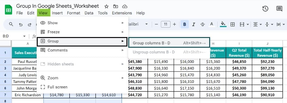
The three chosen columns get grouped.
Step 2: As explained in Step 1, select the entire columns F – H and choose View – Group – Group columns F – H.
The three chosen columns get grouped into a second group.
Step 3: As explained in Step 1, select the entire columns B to I and select View – Group – Group columns B – I.
Thus, the chosen columns get grouped and we can now see multiple layers of grouping.
When we click on the two inner ‘–‘ buttons, one at a time, the respective grouped columns collapse. By doing so, we hide the Q1 and Q2 months’ data while displaying only the Q1 and Q2 total revenue data along with the total half-yearly revenue data.
Finally, when we click on the outer ‘–‘ button, the group of columns B-I collapses, leading to the Sheet displaying only the total half-yearly revenue data.
1. Select the group of rows in question.
2. Choose the Data tab – The Named ranges option to open the Named ranges pane on the right end of the window.
3. Please enter the phrase we want as the name for the specific group of rows in the first field. Next, the second field will show the chosen grouped rows range. Finally, click Done to complete the action.
You cannot group non-contiguous rows or columns in Google Sheets since, in such a scenario, the Group option will be disabled.
Use this Group In Google Sheets Template to follow along with the examples in this article.
Download Excel Template