
What Is IFNA In Google Sheets?
The IF Not Available or the IFNA in Google Sheets is a logical function that checks the dataset for #N/A error. If the error is found, then it returns the specified value in the formula, or else, it will return the cell value as it is. The Google Sheets IFNA helps us handle the “#N/A” error and display them as expressions or an alternate message, that will make the generated reports professional and reliable.
For example, we have a couple of values given below. Let us apply the Google Sheets IFNA function, and view the results.

Select cell B2, enter the formula =IFNA(A2), press “Enter” and drag the formula from cell B2 to B3 using the fill handle.

The output is shown above. For the cell with a value, the formula returned the original value and for the cell with the #N/A error, the formula returned a blank cell. However, if we insert a text or a statement in the formula, then, we will get that as a result, when there is the error, instead of an empty cell.
Use this IFNA In Google Sheets Template to follow along with the examples in this article.
Download Excel TemplateKey Takeaways
- IFNA in Google Sheets helps handle errors smoothly either by displaying the errors or replace it with an alternate expression or message.
- It can be combined with other functions, such as VLOOKUP, HLOOKUP, FILTER, MATCH, etc, to create more sophisticated formulas.
- Since, the IFNA function looks for the #N/A error, all other errors, like the #DIV/0, #NAME!, #REF! etc. will be overlooked. However, to target all errors, we can use the IFERROR function.
- When we are sharing data non–IFNA Google Sheets users, ensure to place a note, if not the other users might not be able to interpret or manipulate the data correctly due to differences in handling missing values.
Syntax
The syntax of the IFNA formula in Google Sheets is,

The arguments of the IFNA formula in Google Sheets are,
- value: It is a mandatory argument. It is the cell value that we must check for the “#N/A” error.
- [value_if_na_error]): It is the expression or the alternate message to be displayed if the “#N/A” error is found. It is an optional argument and it is not provided the formula returns a blank or an empty cell.
How To Use IFNA Function In Google Sheets? (With Steps)
We can use the IFNA In Google Sheets in 2 ways, namely,
- Access from the Google Sheets ribbon.
- Enter in the worksheet manually.
Method #1 – Access from the Google Sheets ribbon –
Choose an empty cell for the output – select the “Insert” tab – click the “Function” option right arrow – click the “Logical” option right arrow – select the “IFNA” function, as shown below.

The “IFNA” formula appears, as shown below. Enter any argument as cell values or cell references, and press “Enter”.

Method #2 -Enter in the worksheet manually –
- Select an empty cell for the output.
- Type =IFNA( in the cell. [Alternatively, type =I or =IFNA and double-click the IFNA function from the Google Sheets suggestions.]

- Enter the arguments as cell values or cell references.
- Close the brackets and press “Enter”.
Examples
Let us consider some IFNA in Google Sheets examples with VLOOKUP(), HLOOKUP(), MATCH(), etc, to understand the results better with an without the IFNA().
Example #1 – IFNA ith VLOOKUP
The dataset given below consists of fruits and their price. We will perform a VLOOKUP with and without the IFNA function.

The steps to perform VLOOKUP with and without IFNA are as follows:
Step 1: Let us find the result of VLOOKUP without IFNA. Select cell E2, enter the formula =VLOOKUP(D2,$A$1:$B$6,2,FALSE), press “Enter” and drag the formula from cell E2 to E3 using the fill handle, as shown below.

Step 2: Let us find the result of VLOOKUP with IFNA. Select cell E7, enter the formula =IFNA(VLOOKUP(D7,$A$1:$B$6,2,FALSE),“Fruit not Found”), press “Enter” and drag the formula from cell E7 to E8 using the fill handle, as shown below.

We can see the output with and without the IFNA function. The VLOOKUP returned the values found and an NA error for values not found. However, the IFNA function returned an alternate expression, i.e., “Fruit not found”, instead of the error.
Example #2 – HLOOKUP with IFNA
The dataset given below consists of employee detains such as their name, ID and department. We will perform a HLOOKUP with and without the IFNA function.

The steps to perform HLOOKUP with and without IFNA are as follows:
Step 1: Let us find the result of HLOOKUP without IFNA. Select cell B9, enter the formula =HLOOKUP(A9,$B$2:$K$4,3,0), press “Enter” and drag the formula from cell B9 to B11 using the fill handle, as shown below.

Step 2: Let us find the result of HLOOKUP with IFNA. Select cell F9, enter the formula =IFNA(HLOOKUP(E9,$B$2:$K$4,3,0),“Employee Details Not Found”, press “Enter” and drag the formula from cell F9 to F11 using the fill handle, as shown below.

We can see the output with and without the IFNA function. The HLOOKUP returned the values found and an NA error for values not found. However, the IFNA function returned an alternate expression, i.e., “Employee Details Not Found”, instead of the error.
Example #3 – IFNA then 0
We can use the formulas mentioned in the previous example to get an alternate expression. However, here we will use the MATCH function with IFNA to get the result of NA error as 0. Consider the dataset of student details such as their names, age, gender, location, etc.

The steps to perform MATCH with and without IFNA are as follows:
Step 1: Let us find the result of MATCH without IFNA. Select cell B10, enter the formula =MATCH(A10,$C$2:$C$6,0), press “Enter” and drag the formula from cell B10 to B12 using the fill handle, as shown below.

Step 2: Let us find the result of MATCH with IFNA. Select cell D10, enter the formula =IFNA(MATCH(D10,$C$2:$C$6,0),0), press “Enter” and drag the formula from cell D10 to D12 using the fill handle, as shown below.

We can see the output with and without the IFNA function. The MATCH returned the position of the values found and NA error for values not found. However, the IFNA function returned 0, meaning value not found and an alternate message, instead of the error.
Example #4 -FILTER with IFNA
We have the dataset that consists of employee names, ID and Department. We will use the Filter function with and without IFNA.

The steps to use FILTER function with and without IFNA are as follows:
Step 1: Let us find the result of FILTER without IFNA. Select cell E10, enter the formula =filter(A4:C4,”ID101″) and press “Enter, as shown below.

Step 2: Let us find the result of FILTER with IFNA. Select cell E5, enter the formula =ifna(FILTER(A3:C3,”Marketing”,”ID101″),”Value Not Found”) and press “Enter, as shown below.

We can see the output with and without the IFNA function. The FILTER returned the NA error. However, the IFNA function returned an alternate expression, i.e., “Value Not Found”, instead of the error.
Important Things To Note
- The second argument for IFNA function is optional and if we do not enter a value for it, by default, the function returns an empty or a blank cell, when it encounters a #N/A error or when the result of a formula is #N/A error.
- Exporting or sharing data with non–IFNA Google Sheets users may be challenging, as they might not be able to interpret or manipulate the data correctly due to differences in handling missing values.
Frequently Asked Questions (FAQs)
We often forget in which category a function falls, here, the “IFNA” function. Then, we can insert the function as follows:
Choose an empty cell – select the “Insert” tab – click the “Function” option right arrow – click the “All” option right arrow – select the “IFNA” function, as shown below.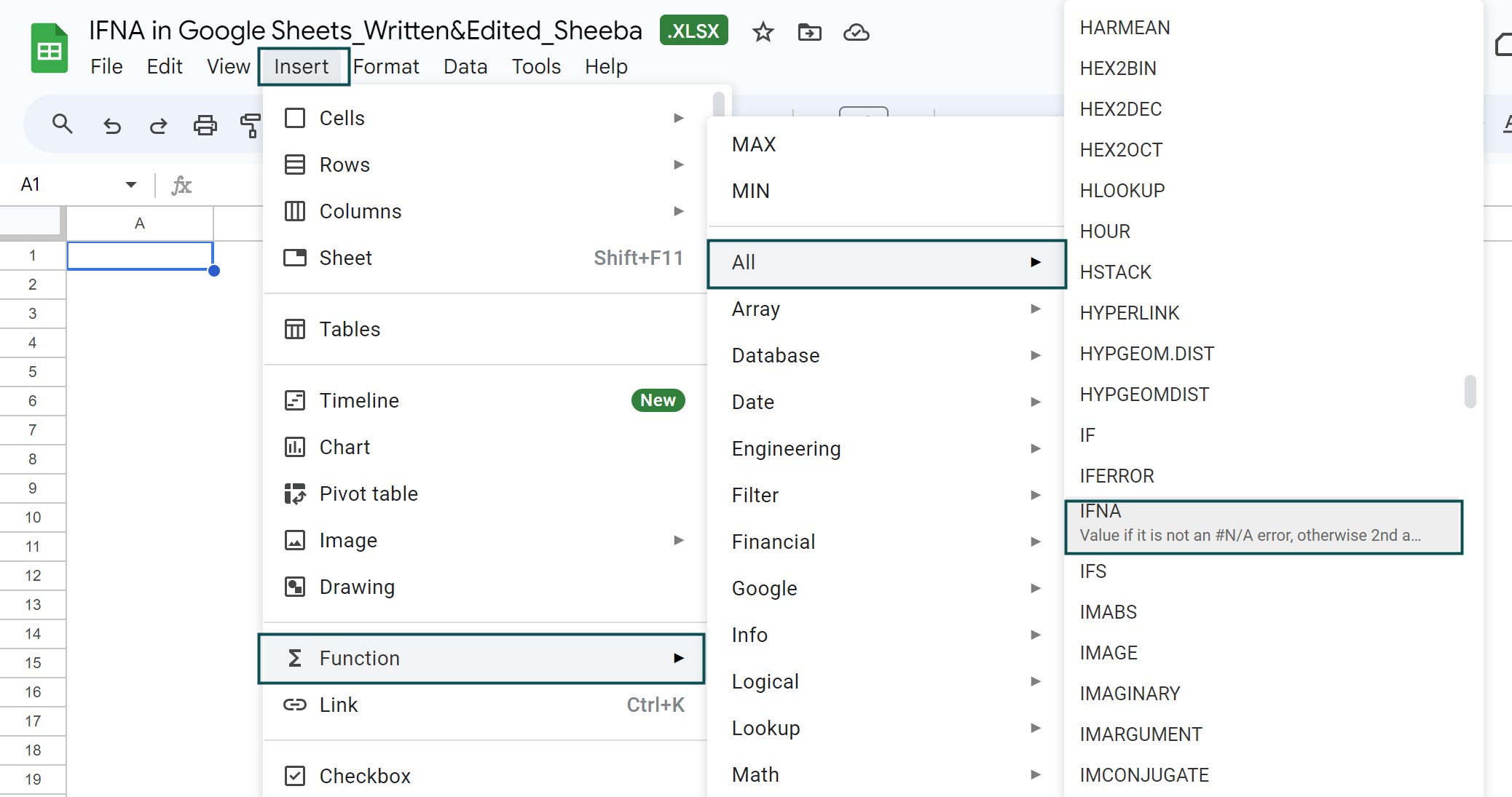
However, as always, entering the function manually is the best way to avoid confusion.
Alternatively, we can find the Functions icon to insert the IFNA function by following the path shown below.
Choose an empty cell – click the “More” option represented by the three vertical dots at the end of the toolbar, as shown below.
A list of icons appears when we click the “More” option. Here, click the “Functions” icon, as shown below.
Here, click the “Functions” option – click the “All” option right arrow – select the “IFNA” function, as shown below.
A few reasons the IFNA in Google Sheets may not work are,
• There is some error other than the #N/A error in the cell value or the result of the formula.
• An alternate expression is not provided and hence the cell is blank or empty. It is still a correct result.
Use this IFNA In Google Sheets Template to follow along with the examples in this article.
Download Excel Template