ISNA In Google Sheets

What is ISNA Function in Google Sheets?

The ISNA function is used to check cells or formulas that give back #N/A errors. The result of ISNA in Google Sheets is a logical value that shows TRUE if a #N/A error is found and FALSE otherwise. In Google Sheets, the ISNA function checks whether a value is an #N/A error. It can be helpful when working with formulas that might result in the #N/A error or looking up non-existing values. It is helpful to handle the error in a specific way, like displaying a custom message or executing some other formula

Let’s say you are using a VLOOKUP function and want to check if the result is #N/A. We used the following function.

=ISNA(VLOOKUP(C1, A1:B5, 2, FALSE))

In this example, the formula checks if the result of the VLOOKUP is #N/A. If it is, the ISNA function returns TRUE; otherwise, it returns FALSE. Here, since do not find “pink” in the table, it returns an #N/A error. So, the formula evaluates to TRUE.

Syntax

The syntax of the ISNA function is as simple as it can get. It just requires one argument.

=ISNA(value)

Here, value is the cell value or formula for which we will check the #N/A errors. It can be a cell reference or a formula or a direct value

To write an ISNA formula in the simplest manner, give a cell reference as its only argument:

=ISNA(A1)

How to Use ISNA Function in Google Sheets?

Using the ISNA function alone is not very beneficial. Often, it is combined with other functions to evaluate the outcome of a particular formula. Let us show you how to use the ISNA function step-by-step manually.

Manually Using the ISNA function

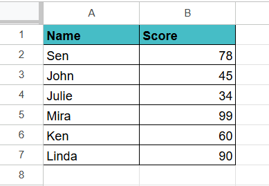
Step 1: Look at the details in the table below. We combine the MATCH function in Google Sheets to find a match and return its relative position otherwise, a #N/A error occurs.

If a lookup value is found, the MATCH function gives its relative position in the lookup array. If not, a #N/A error occurs. To get the result of MATCH, we combine it with ISNA.

Enter the following formula in cell D2.

=MATCH(“Hi”, A2:A5, 0)

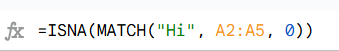
Step 2: Here, we are trying to look up a value “Hi” for a match in Column A, which we obviously do not have. Hence, we wrap the entire function with ISNA manually as follows.

=ISNA(MATCH(“Hi”, A2:A5, 0)). Press Enter.

Step 3: You get TRUE as we get the #N/A error due to the absence of the value. Thus, the function is easy to use manually but its use is enhanced when combined with other functions.

Using the Google Menu bar

• We can also enter the same function using the Google Menu bar.
• Go to the menu bar and click on “Insert” ➝ “Function” ➝ “Info” ➝ “ISNA.”
• Enter the required arguments. Close the bracket and press the “Enter” key.

Examples

Here are some interesting examples of how to use the ISNA function in Google Sheets. By design, the ISNA function can only return two Boolean values. These examples demonstrate how you can use ISNA to manage and display useful information about missing data or discrepancies between different lists in Google Sheets!

Example #1

Step 1: Enter the details required in a table as shown below. Here, we want to find a particular value in a list and print its corresponding value.

Step 2: Now, as explained earlier, using the ISNA function in isolation doesn’t make much sense. Here we write the following function cell C2.

=IF(ISNA(VLOOKUP(1, A2:B6, 2, FALSE)),”Not Present”,”Present”)

Breakdown:

• VLOOKUP is looking for the number 1 and prints its corresponding value in Column B, if present.
• ISNA gives a FALSE if the value is found as there will be no #N/A error.
• ISNA gives a TRUE when the #N/A error is found.
• We use IF to say the student name is present if there is no error(FALSE) and Not present if there is an ISNA error.

Step 3: Press Enter. You get the result Present as the student with Roll No.1 has been found.

Example #2 – Display a custom message when a lookup value is not found

The IF ISNA combination is a useful solution that can be used to search for some value in a set of data. It returns a #N/A error when a lookup value is not found. Let us look at it with this interesting example.

The syntax of the ISNA function with VLOOKUP is as follows:

=IF(ISNA(VLOOKUP(Search), “custom_text”, VLOOKUP(…))

Here, if VLOOKUP results in a #N/A error, the IF will return a custom text, otherwise, you get the VLOOKUP’s result.

In our sample table, we must find the grades of a student. If the student is present, their grades are displayed, else, “Not present” will be displayed.

Step 1: To look up the subjects, we construct this classic VLOOKUP formula:

=VLOOKUP(C2, A2:B7, 2, FALSE)

Step 2: And then nest it in the generic IF ISNA formula discussed above:

=IF(ISNA(VLOOKUP(C2, A2:B7, 2, FALSE)), “Not present”, VLOOKUP(C2, A2:B7, 2, FALSE))

Step 3: Press Enter. You can see that the value we gave is in the table and hence you get the student’s score.

Example #3 – Compare two lists and identify missing items in one list

Here in this example, let us compare two lists and cross-reference them to find missing items. Interesting, isn’t it? Read on to find how we can do it using ISNA in Google Sheets. 

Step 1: Suppose you have two lists. One contains the number of students who scored goals in a tournament. Another list contains all the names of the players in the tournament.

Enter the details in a Google Sheet as shown below. Column A has the names of students who scored a goal. Column D has all the student names who participated in the tournament.

You can use ISNA to identify which names are in Column B and not present in Column A.

Step 2: To find out the above, use the following formula.

=IF(ISNA(MATCH(D2, A:A, 0)), “Did not score”, “Scored goal”)

Explanation:

1. MATCH(D2, A:A, 0) looks for the name in Column D in Column A.
2. If the name is found, MATCH returns the position.
3. If the name is not found, MATCH returns the #N/A error.
4. ISNA checks if the result for #N/A. If it is found, it means the student did not score a goal, so the formula returns “Did not score”.
5. If the name is found in the list, it returns “Scored goal”.

This helps you to identify which students scored a goal of all the participants.  

Now, press Enter.

Step 3: Drag the formula for all the names and check the result.

Important Points to Remember

• The ISNA function specifically handles the #N/A (not available) errors and is more effective for such cases. However, if you need to handle a wide range of errors, use the IFERROR function.
• It helps detect errors when handling huge amounts of data thereby saving time.
• ISNA only returns TRUE for the #N/A error. It doesn’t work for other errors like #DIV/0!, #VALUE!, etc.
• It’s helpful when dealing with lookup functions like VLOOKUP, MATCH, or INDEX where the #N/A error might occur if a value isn’t found.

Frequently Asked Questions (FAQs)

Download Template

This article must help understand ISNA in Google Sheets with its formulas and examples. You can download the template here to use it instantly.

Recommended Articles

Guide to What Is ISNA in Google Sheets. We learn its syntax & how to use it to check cells that give back #N/A errors with examples. You can learn more from the following articles. –

SWITCH Google Sheets Function

Change Google Sheets Row Height

Columns In Google Sheets