
What Is INDEX MATCH Function In Google Sheets?
The INDEX MATCH function in Google Sheets is an INDEX formula containing the MATCH(). The formula helps us look up a value in a table based on the cited row and column number, with MATCH() determining the cell position in the concerned row or column in the formula.
Users can utilize the INDEX MATCH function in Google Sheets when reviewing sales data for conducting a two-way lookup and a left lookup. The function also helps identify the value closest to the desired target value.
Use this INDEX MATCH Function In Google Sheets Template to follow along with the examples in this article.
Download Excel TemplateFor example, the source dataset holds the batch-wise items’ stock availability status data.

We have an item cited in cell F1, for which we must find the stock availability status in cell F2 based on the source dataset.
Then, considering the definition of INDEX MATCH function in Google Sheets explained earlier, we can implement the INDEX-MATCH(), which works like the Excel INDEX MATCH formula, in the target cell. We shall then secure the required data in the target cell.

The INDEX(), which works like the Excel INDEX function, accepts four argument values. The first argument, reference, is the range A2:C11, holding the value we must look up.
Next, the second argument, row, is the MATCH(), which works like the Excel MATCH function. The MATCH() accepts three inputs. The first argument, search_key, is the reference to cell F1 holding the lookup value ITM_15. The second argument, range, value is the range C2:C11, where we must look up the search key ITM_15. The third argument value, search_type, value is 0, indicating that the function must find an exact match for the search key in the unsorted range C2:C11.
Since the MATCH() finds an exact match for the search key ITM_15 in cell C7, the function returns 6 (row 7 of the sheet is row 6 of the range C2:C11)as the required row argument value of the INDEX().
Next, the last argument, column, in the INDEX() is 2 since we require the function to return the target value from the second column (column B) of the reference range of A2:C11. Thus, the INDEX MATCH function in Google Sheets returns the cell B7 (where row 6 of the range A2:C11 and column B meet) value, Stock Unavailable, as the required output.
Key Takeaways
- The INDEX MATCH function in Google Sheets is an INDEX(), with the MATCH() as its second, third, or both arguments. The formula helps in looking up the value in a cell within a table according to the specified horizontal or vertical or both conditions.
- The INDEX-MATCH formula in Google Sheets is useful for carrying out a left, two-way, case-sensitive, or multiple conditions lookup.
- The INDEX-MATCH formula in Google Sheets is a better alternative to the VLOOKUP() since the formula helps in left lookup. Also, the formula works even when we add new columns or move the existing ones to or from the specified lookup range.
Syntax – INDEX Function & MATCH Function
The INDEX function in Google Sheets syntax is the following:

Where,
- reference: The cell range from where the INDEX MATCH function in Google Sheets returns the required target value.
- row: The index of the row to be obtained from the reference range. The argument’s default value is 0.
- column: The index of the column to be obtained from the reference range. The argument’s default value is 0.
While the first argument value is mandatory, the last two are optional in the INDEX().
The MATCH function in Google Sheets syntax is the following:

Where,
- search_key: The value we aim to look for.
- range: The 1-D array that must be searched. If the range’s height and width exceed 1, the MATCH() output is the #N/A! error value.
- search_type: The search type.
- 1: It is the default argument value. In this case, the MATCH() considers that the range values are in ascending order and returns the largest value below or equal to the specified search_key.
- 0: In this case, the MATCH() returns an exact match, with the range values not sorted in any order.
- -1: In this case, the MATCH() considers that the range values are in descending order and returns the smallest value exceeding or equal to the specified search_key.
While the first two argument values are mandatory, the last is optional in the MATCH().
Then, adhering to the definition of INDEX MATCH function in Google Sheets explained previously, we can apply any of the following INDEX-MATCH() formulas according to our requirements.


How To Use INDEX MATCH Function In Google Sheets?
The steps for using INDEX MATCH function in Google Sheets are as follows:
- Click a cell to choose it for displaying the output.
- Enter the INDEX MATCH formula, mentioned in the previous section according to the requirements.
- Press Enter to view the value formula returns in the chosen cell.
Examples
Check out the following illustrations explaining the practical ways of using INDEX MATCH function in Google Sheets.
Example #1
The source dataset contains the top ten tech companies and their stock prices.

We must determine the rank of the tech company cited in cell F1 based on the source dataset and showcase the output in cell F2.
Then, we can use the INDEX-MATCH() in the target cell to fetch the required data.
Step 1: Choose cell F2, enter the INDEX-MATCH(), and press Enter.
=INDEX(A2:C11,MATCH(F1,B2:B11,0),1)

The INDEX() takes four argument values. The first argument, reference, is the range A2:C11, containing the value we must search and from where we must return the target value.
Next, the second argument, row, is the MATCH(). The MATCH() takes three inputs. The first argument, search_key, is the reference to cell F1 holding the lookup value TSMC. The second argument, range, value is the range B2:B11, where we must search the search key TSMC. The third argument value, search_type, value is 0, denoting that the function must locate an exact match for the search key in the unsorted range B2:B11.
The MATCH() locates an exact match for the search key TSMC in cell B8. So, the function returns 7 (row 8 of the sheet is row 7 of the range B2:B11)as the required row argument value of the INDEX().
Next, the last argument, column, in the INDEX() is 1 since we require the function to return the target value from the first column (column A) of the reference range of A2:C11. Thus, the INDEX-MATCH() returns the cell A8 (where row 7 of the range A2:C11 and column A meet) value, TC_7, as the required output.
Example #2
We shall see an example of a case-sensitive lookup using the INDEX-MATCH() in Google Sheets.
The source dataset lists the top ten US cities based on the median home prices and the average annual salaries.

However, a few cities occur twice, with one occurrence showing the city name with its first character in lower case and the other in upper case.
The requirement is to display the median home price value for the US city specified in column E, considering their case. Assume cells F2:F3 are the target cells.
Then, we must apply the INDEX-MATCH() with the FIND(), similar to the Excel FIND function, in the target cells to acquire the required data.
Step 1: Select cell F2, enter the following formula, and press Enter.
=INDEX($B$2:$B$12,MATCH(1,FIND(E2,$A$2:$A$12)),0)

Next, utilizing the fill handle option, feed the formula in cell F3.

Please note that we use absolute reference, which is similar to the Excel absolute reference, when referencing the ranges in the formula. It is only to make it easier to apply the formula in the second target cell.
Let us check the cell F3 formula to understand its logic.
First, the FIND() locates the first case-sensitive occurrence of the text specified in cell E3, Miami, in the range A2:A12. The function finds the value in cell A5. So, the FIND() output is an array where all the values are the #VALUE! error, except for the value at the fourth position being 1. The array indicates that the function did not find a match in any cell in the range A2:A12, except in one cell, A5, which is the fourth cell in the range A2:A12.
Next, the MATCH() tries to find a match for the value 1 in the array the FIND() returns, which it finds at the fourth position.
So now, the INDEX() inputs are the cell range B2:B12, row number 4, and column number 0. The column index is 0 since the reference range contains only one column, which contains the potential target value. Thus, the function returns the value in the cell where row 4 of the range B2:B12 and column B meet, which is the cell B5 value of $608,742.
Example #3
Let us understand the INDEX MATCH function in Google Sheets multiple criteria with an example.
The source dataset contains the sales data of sales representatives across different zonal offices of a firm.

We must display the sales data in cell K2 for a representative in a specific zone and month, chosen from the respective lists in cells H2:J2.
Step 1: Choose cell H2 and Data – Data Validation.

The Data validation rules pane will appear, where we must click the + Add rule option.

Step 2: The Apply to range field shows the chosen cell address. Next, set the Criteria field as the Dropdown (from a range) option.

Next, click the box icon under the Criteria field to open the window where we must update the range containing the values we must include in the dropdown list in the chosen cell. Here, we shall select the range A3:A10 containing the zones to list the zones in the cell H2 dropdown list.

Click OK and then Done.

Step 3: Choose cell I2 and click the + Add rule option to create the next rule.

Iterate the process explained in Step 2 to list the sales representatives in the cell I2 dropdown list. In this case, the cell range to update under the Criteria field is B3:B10.


Click OK and Done.

Step 4: Choose cell J2 and click the + Add rule option to create the next rule.

Iterate the process explained in Step 2 to list the months in the cell J2 dropdown list. In this case, the cell range to update under the Criteria field is C2:F2.


Next, click OK and Done.


Once all the rules are created, close the Data validation rules window.
Step 5: Choose cell K2, enter the INDEX MATCH function in Google Sheets multiple criteria, and press Enter.
=INDEX(A3:F10,MATCH(1,(H2=A3:A10)*(I2=B3:B10),0),MATCH(J2,A2:F2,0))

Step 6: Click the cell H2 dropdown button to set the required zone. We shall click South to set it as the zone.

Next, click the cell I2 dropdown button to set the required sales representative. We shall click Jacob to set it as the sales representative.

Next, click the cell J2 dropdown button to set the required month. We shall click Mar to set it as the month.

Once we choose the required options from the respective dropdown lists, the INDEX-MATCH() in cell K2 will show the corresponding sales figure of $2,500 as the required output.

First, the expressions (H2=A3:A10) and (I2=B3:B10) return arrays of TRUEs and FALSEs. The value in the first array will be TRUE when the corresponding cell A contains the zone as South. Otherwise, the array value will be FALSE. Next, the value in the second array will be TRUE when the corresponding cell B contains the sales representative as Jacob. Otherwise, the array value will be FALSE.
Next, once we multiply the two arrays, the result will be an array of 1s and 0s. The value in the resulting array will be 1 when the values at the same position in the two input arrays are 1. Otherwise, the value in the resulting array will be 0.
Next, the first MATCH() looks for an exact match for the value of 1 in the resulting array of 1s and 0s, which it finds at the 6th position in the array. So, the function returns the value of 6 as the output.
Next, the second MATCH() looks for an exact match for the value of Mar in the range A2:F2, the column headings. The function finds the match in cell E2. So, it returns 5 since the cell is the fifth one in the range A2:F2.
So, the INDEX() inputs are the reference range A3:F10, the row argument value is 6, and the column argument value is 5. Thus, based on the input values, the INDEX() returns the value in the cell, where row 6 and column E of the range A3:F10 meet, which is the cell E8 value of $2,500.
Important Things To Note
- Ensure the reference range supplied to the INDEX() in the INDEX MATCH function in Google Sheetsis correct. Otherwise, the formula output will be the #NUM! error.
- Ensure the row and column arguments of the INDEX() in the INDEX MATCH formula in Google Sheetspoint to a cell within the given array. Otherwise, the formula output will be the #REF! error.
- Ensure the range supplied to the MATCH() in the INDEX MATCH formula in Google Sheetsis correct. Otherwise, the formula output will be the #N/A! error.
Frequently Asked Questions (FAQs)
You can INDEX and MATCH multiple columns in Google Sheets, as explained below with an example.
The source dataset shows employees’ IDs, names, designations, and their appraisal statuses.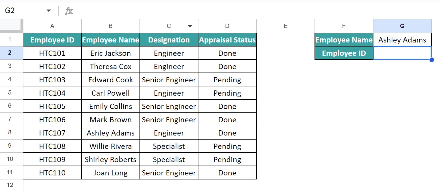
We must show the ID of the employee, cited in cell G1, based on the source dataset. We shall consider cell G2 as the target cell.
Then, the process is as follows:
Step 1: Choose cell G2, enter the INDEX-MATCH(), and press Enter.
=INDEX(A2:D11,MATCH(G1,B2:B11,0),MATCH(F2,A1:D1,0))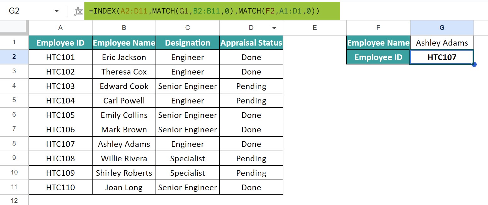
The first MATCH() searches for the exact match for the employee name, cited in cell G1, Ashley Adams, in the range B2:B11. The function finds the match in cell B8. So, the function returns 7 (row 7 of the range B2:B11 is row 8 of the sheet) as the row argument value of the INDEX().
The second MATCH() searches for the exact match for the field, cited in cell F2, Employee ID, in the range A1:D1. The function finds the match in cell A1. So, the function returns 1 (column A is the first column of the range A1:D1) as the column argument value of the INDEX().
So, the INDEX() inputs are the reference range A2:D11, the row argument value is 7, and the column argument value is 1. Thus, based on the input values, the INDEX() returns the value in the cell, where row 7 and column A of the range A2:D11 meet, which is the cell A8 value of HTC_107.
You should prefer INDEX MATCH over VLOOKUP in Google Sheets due to the following reasons:
• The INDEX-MATCH function enables us to do a left, two-way, case-sensitive, and vertical using multiple criteria lookup.
• The INDEX-MATCH function works well even if we make column changes in the lookup range.
There is something better than INDEX MATCH in Google Sheets, which is the XLOOKUP built-in function in Google Sheets.
Use this INDEX MATCH Function In Google Sheets Template to follow along with the examples in this article.
Download Excel TemplateRecommended Articles
Continue with these related resources when you want the next practical step in this topic.
- LOOKUP in Google Sheets
- HLOOKUP In Google Sheets
- VLOOKUP Table Array In Google Sheets
- VLOOKUP True In Google Sheets
- MATCH Function In Google Sheets
Explore the full Google Sheets Lookup Functions guide or browse Google Sheets Resources.