Macros in Excel

What are Macros In Excel?

Macros is a piece of code that hold the set of instructions to perform a certain set of operation in Excel. It is a program code stored in an Excel workbook to perform a pre-defined sequence of tasks. After we create the macro code, we can save this macro code. Then, we can reuse it whenever we have to perform the same set of tasks. Hence, we can use macros to repeat all the time-consuming tasks and save a lot of time with just a click of a button.

Often we confuse Macros with VBA. But, there is a difference between these two. A macro is a piece of code written using the Visual Basic for Applications (VBA) programming language.

Enable Macros Using Developer Tab

Macros is available under the Developer tab in Excel.

How To Create Macros In Excel?

The method to create macros in Excel is as simple as recording a video. So, let us have a look at a simple way of creating a macro in Excel.

We can create macros in Excel in 2 ways. The first one is by recording a macro, and the second one is using Visual Basic Editor.

Recording a Macro: This doesn’t require any programming language experience to start with. The code records all the activities that we do in Excel.

Therefore, by enabling record macro, we can record each and every moment that we do in Excel and can run the same record whenever we want to perform the same activity.

Once we stop the recording, Excel will no longer record activities. However, we can see and edit the codes for the recorded macro in the Visual Basic Editor and make some amendments.

Example #1 – Create Macro For Quick Formatting

For instance, we have the following quarterly sales information in Excel.

Assume, we need to apply some formatting for the total row of each quarter, and we have to do this 4 times. However, while applying the formatting for the first quarter, we will record the macro, and then we will reuse the same macro for other quarters as well.

• Step 1: First, select the 1st quarter total range from A5:B5.

• Step 2: Next, go to the Developer Tab and then, click on the option Use Relative References.

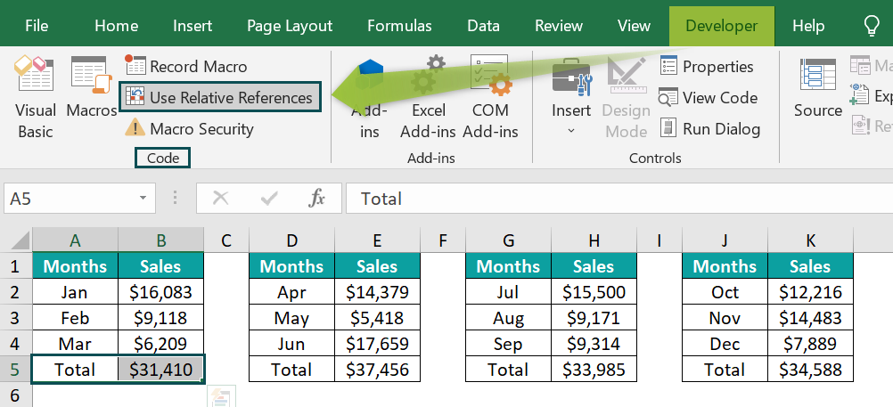
Note: We choose Use Relative References in the current selection (A5:B5) reference because it is useful to select other cells as well. Remember that the range A5:B5 will be treated as selected cells and not as range.

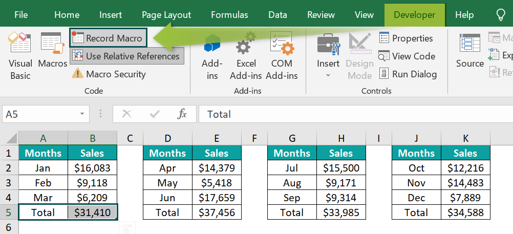
• Step 3: Then, click on Record Macro now.

• Step 4: Now, Record Macro window will appear. In this window, we need to give a name to the macro and give the name as Cell_Formatting.

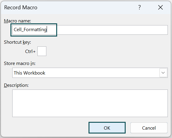
• Step 5: Then, click on OK. Now, all the activities that we do in this workbook will be recorded and written in code.

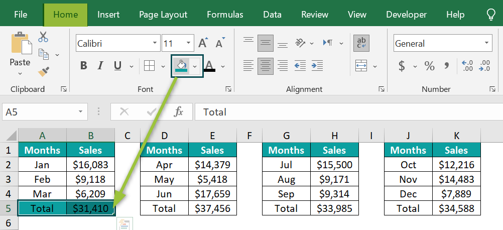
• Step 6: Now, apply formatting as background fill cell color for the selected cell range A5:B5.

• Step 7: Next, change the font color to White.

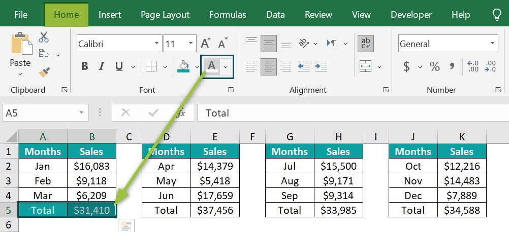
• Step 8: Similarly, apply Bold formatting for fonts.

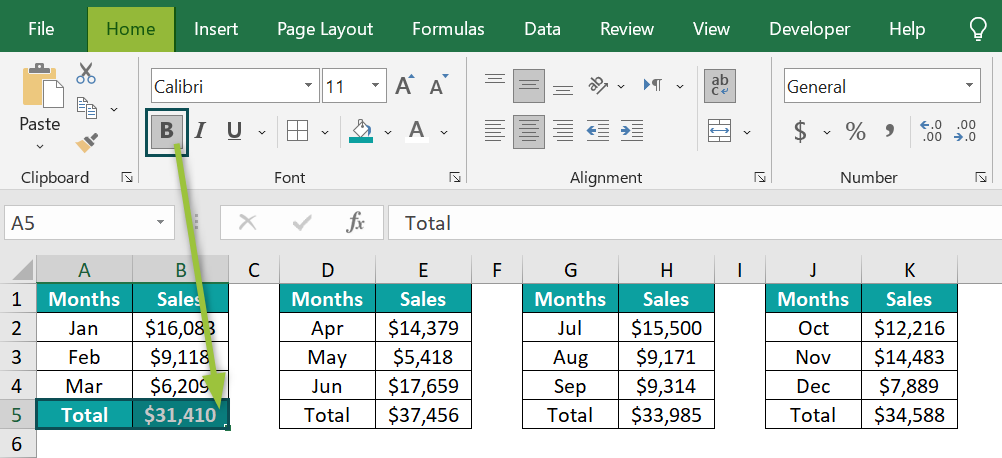
Note: We can press the bold shortcut keys Ctrl + B.

• Step 9: Now, all the formatting has been applied to the total column. Under the Developer tab, click on Stop Recording.

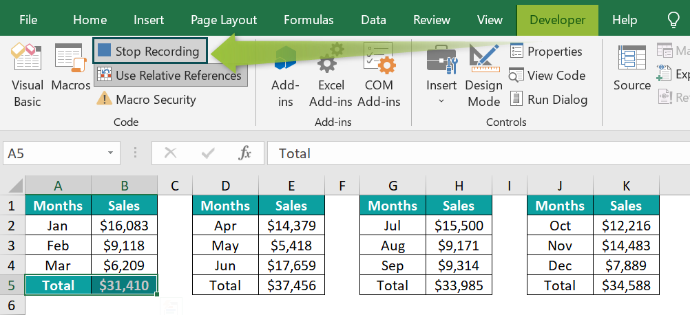
• Step 10: Next, Excel will no longer record the activities we do in Excel.

Now, we need to apply the same formatting for the remaining 3 quarters as well. Now, select all the 3 quarters total by using Ctrl + Click.

• Step 11: Next, go to the Developer tab and then, click on Macros.

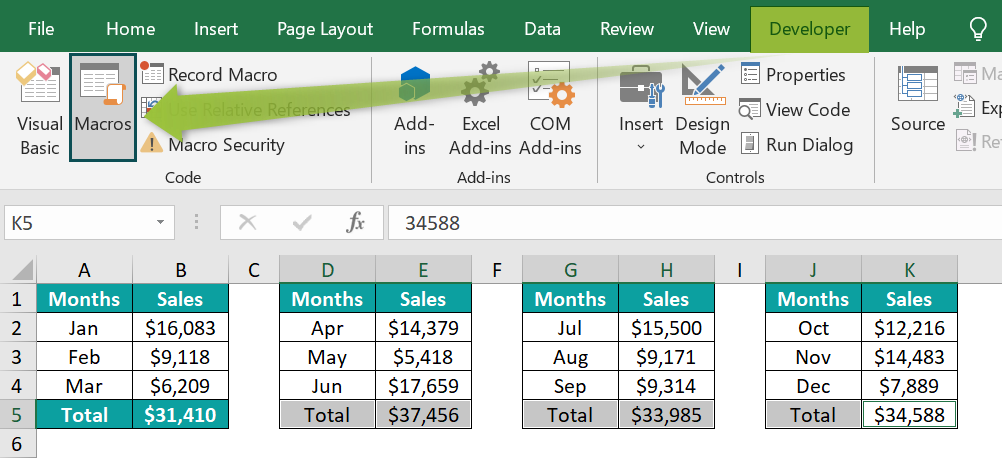
• Step 12: This will bring the list of macros created in this workbook. Now, select the macro name Cell_Formatting and then, click on the Run button.

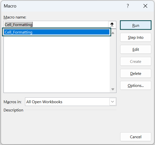
As soon as we click on the Run button, all the selected cells will be formatted exactly the same as the first quarter total formatting.

As soon as we click the button, all the selected cells become formatted.

Example #2 – Arrive Status

For instance, we have the following fruits list and their price in an Excel spreadsheet.

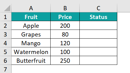
In the status column, we need to arrive at the values based on the cost of the fruit.

• If the price is greater than 100, then the status will be “Expensive”.
• If the price is less than 100, then the status will be “Reasonable”.

While doing this exercise, let us record the macro.

• Step 1: To begin with, select the cell range from C2:C6.

• Step 2: Next, go to the Developer tab and then, click on the option Use Relative References.

• Step 3: Then, click on Record Macro.

• Step 4: Now, Record Macro window tab will appear. In this window, we need to give a name to the macro and then, give the name Status.

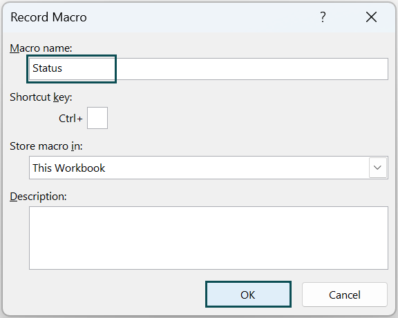
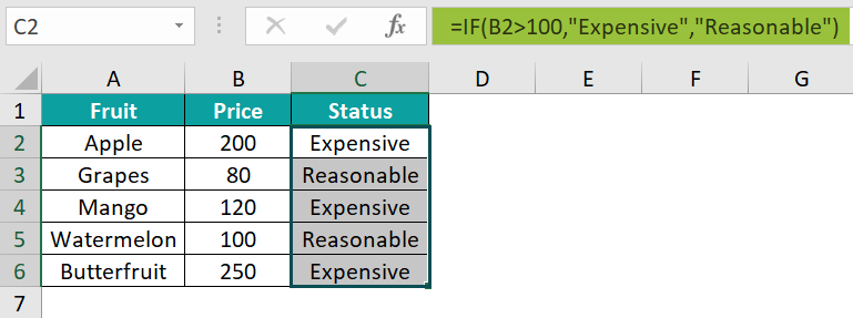
• Step 5: Now, Excel starts the recording of all the activities. Enter the IF Excel formula as shown in the following image.

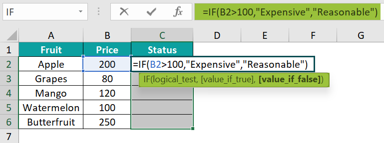
Explanation of the formula: IF condition checks if the price of the values in the price column >100, if yes then it will return the value as Expensive, or else it will return Reasonable.

• Step 6: Now, press Ctrl + Enter key to apply the formula to all the selected cells.

• Step 7: Next, go to the Developer tab and then, click on Stop Recording.

• Step 8: Now we have another list of fruits like the following.

For this list of fruits as well, we need to arrive at the status column based on the price of the fruit

• Step 9: Next, choose cell range G2:G6.

• Step 10: Now, go to the Developer tab and then, click on Macros.

• Step 11: From the macros list, choose Status macro and click on Run.

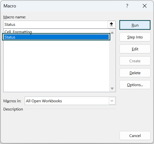
As soon as we run the macro, it will automatically arrive at the values in the selected status column.

Like this, we can automate all the repetitive tasks and make the work easier.

Adding The Macro Button

Once the macro has been created, we cannot force the user to go to the Developer tab every time to run the macro. What we can do is, we can add the button or shape to the Excel worksheet and then assign the macro to the shape. So, whenever the user clicks on the shape macro will be executed, and the task will be performed.

For instance, going back to Example #1, we have created the cell formatting macro.

To begin with, go to the Insert tab and draw the Rectangular shape.

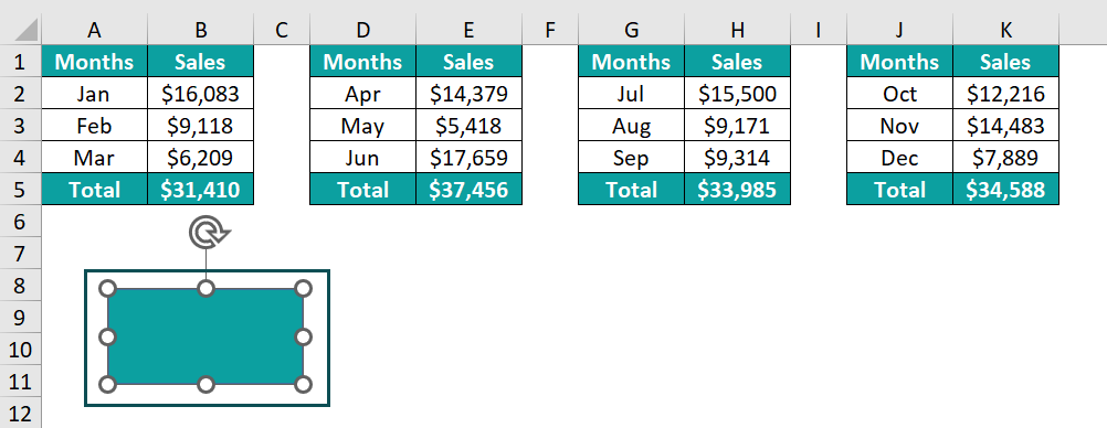
Next, right-click on the shape and then, click on Assign Macro.

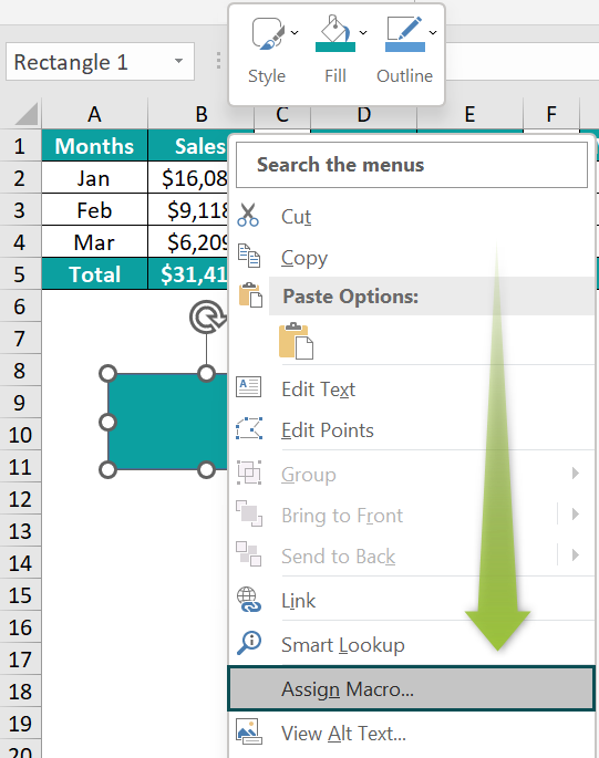
This will bring the macro list window. Choose the appropriate macro and click on OK.

Now, macro has been assigned to the shape.

Again, right click on the shape and click on Edit Text.

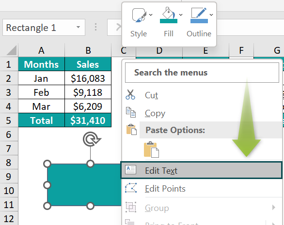
Enter the text as Format Total Rows.

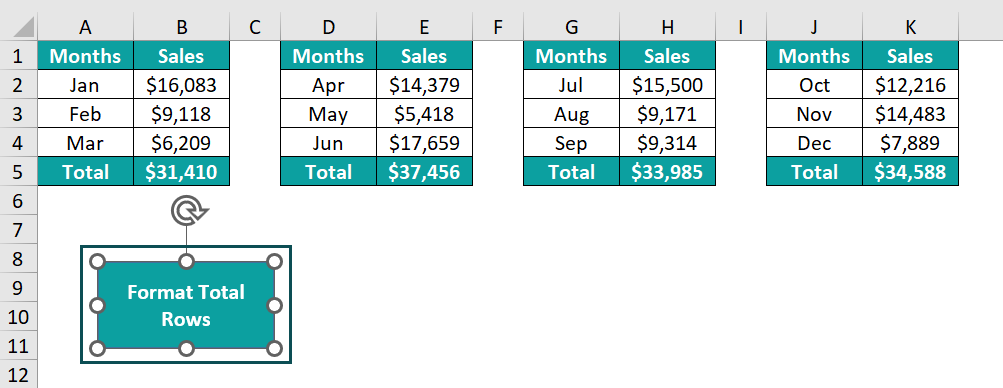
Now, the formatting macro is assigned to the shape.

Remove formatting to test it.

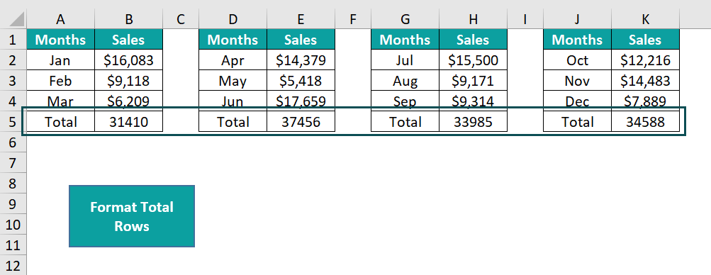
Now select all the total rows and click on the macro assigned shape.

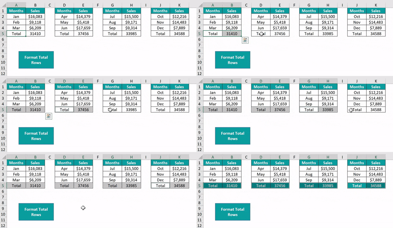
In this way, we can assign macros to the shapes and allow the user to use the macros with just a click of a button.

How To View The Code Of Macros?

Once the macro is created, we can see the code of the macro in the Visual Basic Editor. Go to the Developer tab and click on Visual Basic.

Now we can see the Visual Basic Editor window.

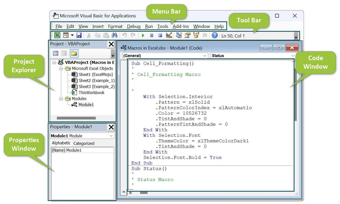
• Menu Bar: Here we have all the options to work with the visual basic editor. This is the ribbon we have in Excel.

• Tool Bar: In Excel, we have a quick access toolbar, this is exactly the same in visual basic editor as well.

• Project Explorer: Here we have a list of all the workbooks and worksheets that belong to it. For instance, we have a workbook named “12. Macros in Excel” and all the worksheets below.

• Properties Window: In this window, we can change the properties of all the objects like workbooks, worksheets, etc.…

• Code Window: This is where all the macro codes will be created. We have created two macros named “Cell_Formatting” and “Status” in this article. We can see the code for these two macros.

How To Save The Recorded Macro In Excel?

All the macro-coded Excel workbooks should be saved in the extension of “macro-enabled extension (.xlsm)”.

The default file extension for Excel is .xlsx and this extension cannot hold macro codes. If we try to save the file after recording the macro code, we will get the following warning message box.

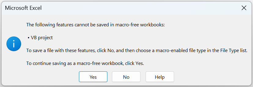
The current workbook is a macro-free workbook, to save a file with these features. We need to save it as the macro-enabled workbook.

In the workbook, press the save as shortcut key F12 and choose the file type as Excel Macro-Enabled Workbook.

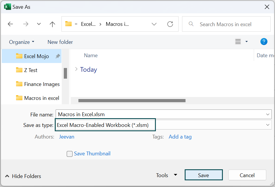
Click on Save. Now, the file is named with the extension as xlsm.

How To Enable “Macro Security Settings”?

With the default setting of Excel, when we open the workbook that contains the macros, we will get the yellow security warning message bar that appears just above the formula bar.

Click on Enable Content and Excel will ask whether we trust the source file that contains the macros.

We need to enable the macro in the background.

• Step 1: Go to the File tab.

• Step 2: Click on Options.

• Step 3: Click on Trust Center in the Excel Options window and then click on Trust Center Settings.

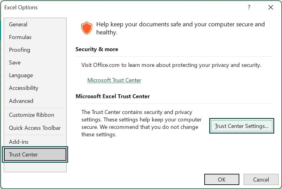
• Step 4: This will open the Trust Center window. Choose Macro Settings.

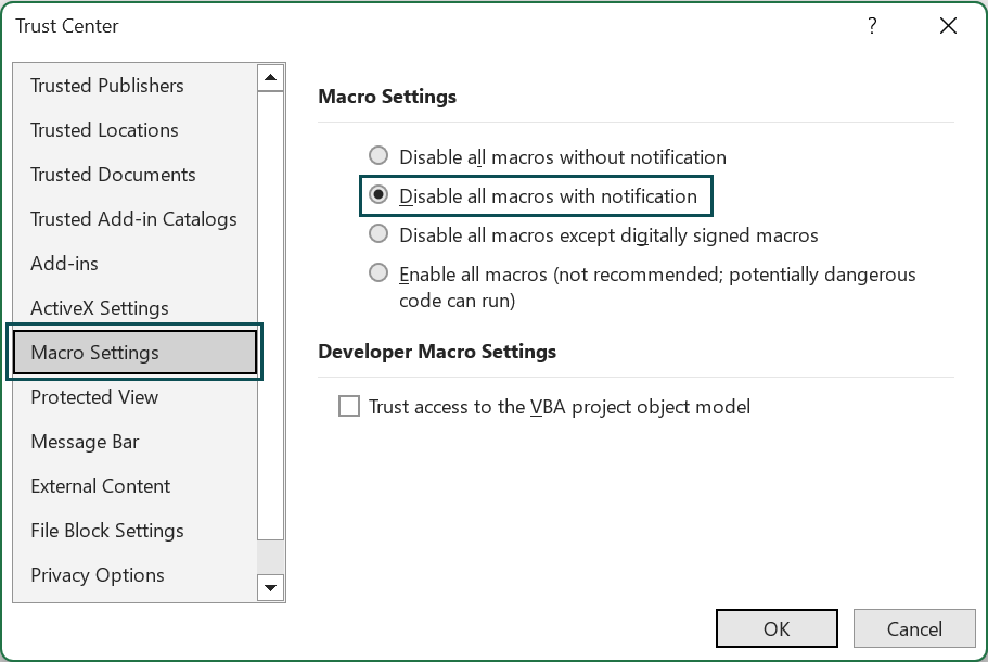
As we can see, by default macros are disabled here.

• Step 5: Choose the option Enable VBA macros (not recommended; potentially dangerous code can run).

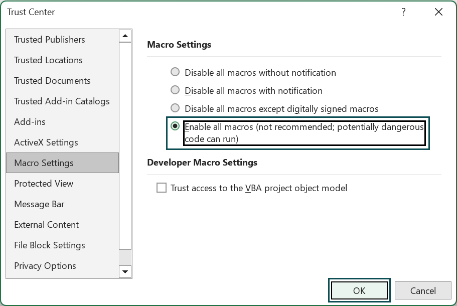
• Step 6: Click on OK in the next windows and macros should work fine now.

Macros In Excel Not Working

One of the primary reasons for macro not working in Excel workbook is because of the following reasons.

• Macros are disabled in your Excel workbook. Enable it to use it.
• There must be a wrong in the code. Use step into to check the codes line by line.

Important Things To Note

• The Developer tab, by default, is not enabled in any Excel.
• Macro is a piece of code written or recorded to perform a certain set of tasks.
• Use relative reference to apply the same task performance of macro to any other selected range of cells.
• Macros are by default disabled in Excel because of dangerous external sources may hamper the file and data.
• While naming a macro, space or any other special characters should not be included. However, we can use the underscore (_) to name a macro.

Frequently Asked Questions (FAQs)

Download Template

This article must help understand Macros in Excel with its features and examples. You can download the template here to use it instantly.

Recommended Articles

This has been a guide to Macros in Excel. Here we learn how to enable, create, record & save Macros, their security settings, examples & downloadable template. You can learn more from the following articles – 

• VBA Macros
• Excel Extensions
• Formula Auditing in Excel