
What Is Marksheet Format In Excel?
Marksheet in Excel is created in an Excel workbook to maintain a cumulative data for present and future analysis. It helps us keep track of the performances of the employees in a company, students in an educational organization, etc.
An Excel Marksheet format is an automated Marksheet that gives us the required results when we modify or update the existing data, or add new data.
Use this Marksheet In Excel Template to follow along with the examples in this article.
Download Excel TemplateKey Takeaways
- The Marksheet in Excel is created to calculate the result of the students.
- Excel functions such as IF, SUM, AVERAGE, COUNTIF, ROUND, etc., are used to calculate the results, like finding the total, average, and count of students falling under specific criteria, etc., using Marksheet format and formulas.
- We can provide an alternative output instead of the default “True” or “False” using the conditional functions such as IF() and COUNTIF(), as we saw in the examples like output as Pass or Fail, Promoted or Distinction, etc.
How To Make Marksheet In Excel Format?
We can Make Marksheet In Excel Format using the following methods, namely,
- SUM function.
- Comma Method.
- Colon Method (Shift Method).
- AVERAGE function.
- ROUND function.
- IF function.
- COUNTIF function
#1 – SUM Function
It adds the selected numeric cell values and returns the total value. Its syntax is,
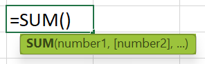
- SUM function – Comma Method – In this method, we enter the cell values separately in the formula using commas.
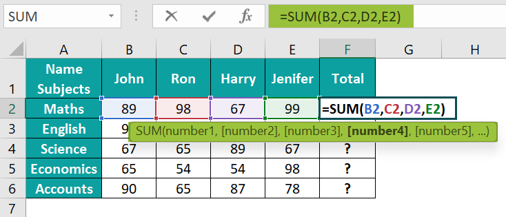
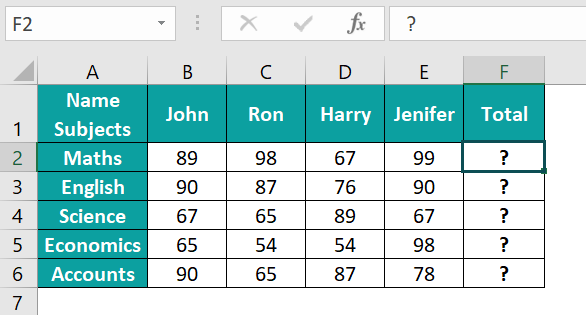
The following example depicts the marks of the subjects of the students of a class, and we will calculate the total marks using the Excel SUM Function Comma Method.
The steps to evaluate the values using the Excel SUM Function Comma Method are as follows:
- Step 1: Select cell F2.

- Step 2: Next, we will enter the Excel SUM Formula in cell F2.
- Enter the value of ‘number1’ as B2, i.e., the sum values in cell B2.
- Enter the value of ‘number2’ as C2, i.e., the sum values in cell C2.
- Enter the value of ‘number3’ as D2, i.e., the sum values in cell D2.
- Enter the value of ‘number4’ as E2, i.e., the sum values in cell E2.
Therefore, the complete formula is =SUM(B2,C2,D2,E2) in cell F2.
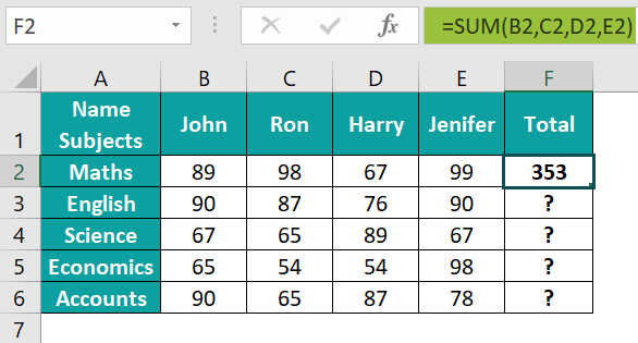
- Step 3: Press the “Enter” key. The result is “353” in the image below.
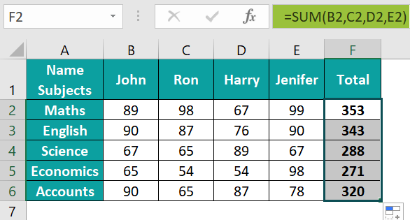
- Step 4: Drag the formula from cell F2 to F6 using the fill handle in excel. The output is shown below.
- SUM function – Colon Method (Shift Method) – In this method, the cell values are entered by selecting the cell range or dragging the cursor on the required cells.
Using the same example as above, we will calculate the marks of the subjects of the students of a class and the total marks using the Excel SUM Function Colon Method.
The steps to evaluate the values using the Excel SUM Function Colon Method are as follows:
- Step 1: Select cell F2.
- Step 2: Next, we will enter the Excel SUM Formula =SUM(B2:E2) in cell F2.

- Step 3: Press the “Enter” key. The result is “353” in the image below.

- Step 4: Drag the formula from cell F2 to F6 using the fill handle. The output is shown below.
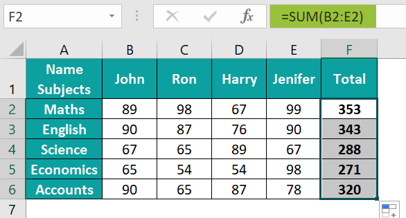
Output Observation: Hence, both the methods of the SUM function, i.e., the Comma Method and the Colon Method, gives the same output.
#2 – AVERAGE Function
It returns the average of the selected numerical values. The values can be numbers, percentages, or time. The function first calculates the sum of the values, and divides it by the count of the values of the list.

For instance, the data below depicts the marks of the subjects of the students of a class, and we will calculate the average marks using the Excel AVERAGE Function.
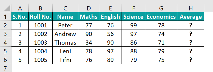
The steps to evaluate the values using the AVERAGE Function are as follows:
- Step 1: Select cell H2, and enter the formula =AVERAGE(D2:G2).

- Step 2: Press the “Enter” key. The result is “82.5” in the image below.
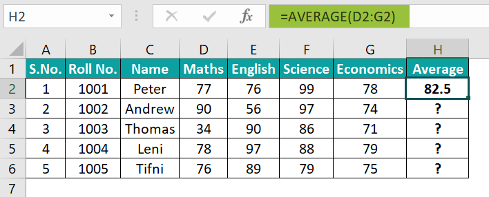
- Step 3: Drag the formula from cell H2 to H6 using the fill handle. The output is shown below.

#3 – ROUND Function
It is used to round up the numerical data according to the number of digits assigned to round the values.

ROUND functions Arguments Explanation
- number: It is the numerical value we want to round up or down. It is a mandatory argument.
- num_digits: It is the number of digits we want to round up. It is a mandatory argument.
The following example depicts the marks and average marks of the subjects of the students of a class, and we will calculate the round value of the average marks using the Excel ROUND Function.
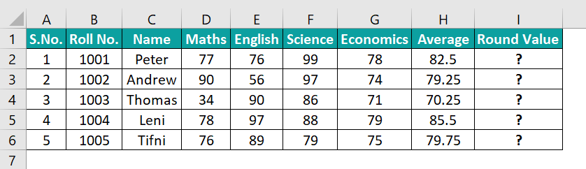
The steps to evaluate the values using the Excel ROUND Function are as follows:
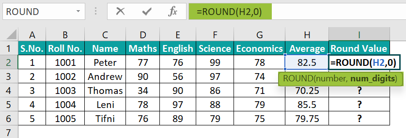
- Step 1: Select cell I2, and enter the formula =ROUND(H2,0).
- Step 2: Press the “Enter” key. The result is “83” in the image below.
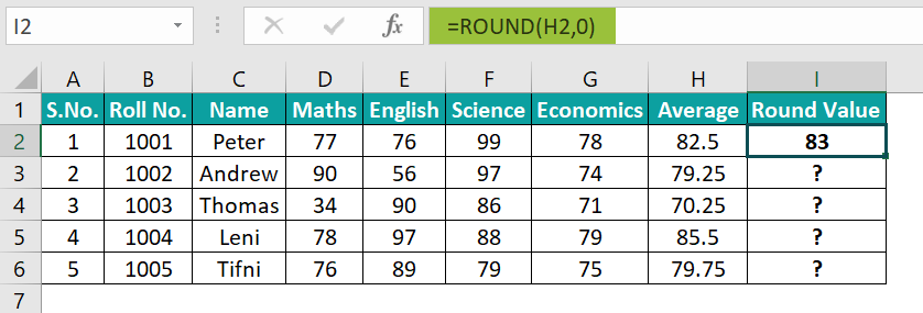
- Step 3: Drag the formula from cell I2 to I6 using the fill handle. The output is shown below.

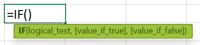
#4 – IF Function
It tests the logical conditions and gives the output as true or false. In addition, it performs analytical tests for the given data using mathematical operators. The argument can have desired output other than true and false.
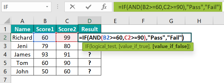
The following example depicts the scores of two subjects of the students of a class, and we will evaluate whether they are passing or failing using the Excel IF Function.

The steps to evaluate the values using the Excel IF Function are as follows:
- Step 1: Select cell D2, and enter the formula =IF(AND(B2>=60, C2>=90), “Pass,” “Fail”)
[Note: The ‘logical test’ value is B2>=60 AND C2>=90, i.e., the condition values of cells B2 & C2. ]
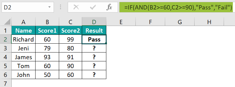
- Step 2: Press the “Enter” key. The result is “Pass” in the image below.
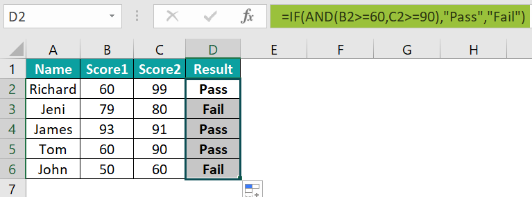
- Step 3: Drag the formula from cell D2 to D6 using the fill handle. The output is shown below.
#5 – COUNTIF Function
It counts all the cells with cell values in the range as specified by the conditions.
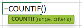
COUNTIF functions Arguments Explanation
- range: It is a range on which the criteria argument is applied. It is a mandatory argument.
- criteria: It is a condition applied to the range of values argument. It is a mandatory argument.
The following example depicts the annual scores of the subjects of the students of a class, and we will whose score is greater than 80 using the Excel COUNTIF Function.
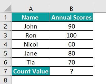
The steps to evaluate the values using the Excel COUNTIF Function are as follows:
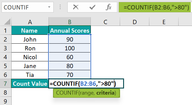
- Step 1: Select cell B7, and enter the formula =COUNTIF(B2:B6,“>80”), i.e., the ‘range’ value is B2:B6, and the ‘criteria’ value is ‘>80’.
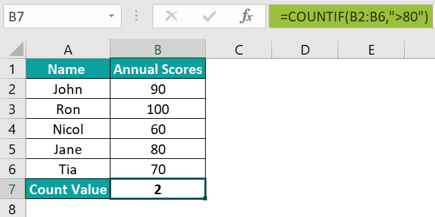
- Step 2: Press the “Enter” key. The result is “2”, i.e., in the cell range B2 to B6, there are 2 cells greater than 80 [cell B2 and B3].
Important Things To Note
- All the formulas used should be written in the correct syntax, or else we will get the “#NAME?” error.
- For entering any text in the function, we should use double quotes (“ ”) as we have used while writing “Pass,” or “Fail,” etc, in the IF and COUNTIF function examples.
- If the dataset consists of non-numeric values in the Marksheet, the formulas ignore them and finds the total of the other numeric values, irrespective of the functions used.
Frequently Asked Questions (FAQs)
Following are the steps to create a Marksheet in Excel.
1) Insert Personal Details. The first part of our mark sheet contains the student details.
2) Insert the Subject Names as column Headers.
3) Insert respective Marks of the subjects of individual students.
4) Insert Subject wise Grades
5) Calculate Total Marks using the formulas.
6) Calculate the Result and display the same.
To calculate the grade, we need to,
• Add up all scores,
• Divide by the total number of exam points, and
• Multiply by the weighted percentage.
• Then calculate the percentage for the project, and add the two totals together to get the final grade.
The following example depicts the annual scores of the students of a class, and we will evaluate whether they have got Distinction using the Excel IF Function.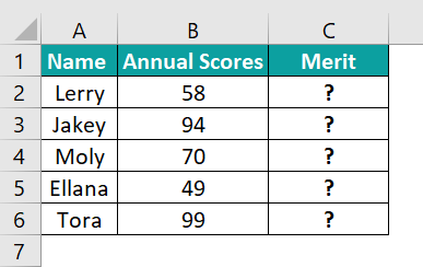
The procedure to evaluate the values using the Excel IF Function is,
• Select cell C2.
• Enter the formula =IF(B2>=80), “Distinction,” “Promoted”)
• Press the “Enter” key.
• Drag the formula from cell C1 to C6 using the fill handle.
[Note: The ‘logical test’ value is B2>=80 AND C2>=90, the ‘value if true’ value is ‘Distinction,’, and the ‘value if false’ value is ‘Promoted,’]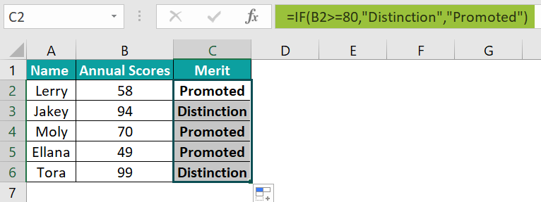
The output is shown above, i.e., student details in cells C2, C4, and C5, are promoted, and the student details in cells C3 and C6, are promoted with distinction.
Use this Marksheet In Excel Template to follow along with the examples in this article.
Download Excel Template