What Is Split Cells In Excel?
The Split Cells in Excel is a feature that separates the cell data into two or more different cells. It helps users format huge data, thus making it easy to filter, sort, or find specific data in the worksheet. It is one of the options available under the Data Tools group of the Data tab.
Let us understand how split cells function is used in Excel with an example. In the below table, column A shows the names of people, and column B shows their age and date of birth. So, we need to use split cells in excel to divide the data into columns C and D, respectively.
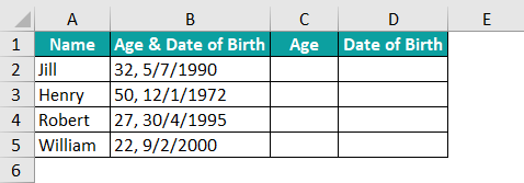
The steps to split cells in excel are as follows:
Step 1: To begin with, choose the cell range B2:B5.
Step 2: Then, click on the Data tab.
Select the Text to Columns option from the Data Tools group.
Step 3: First, the Convert Text to Columns Wizard – Step 1 of 3 window appears.
Select the Delimited radio button and click Next.
Step 4: Next, the Convert Text to Columns Wizard – Step 2 of 3 window pops up.
Choose the Space checkbox and click Next.
Step 5: Lastly, the Convert Text to Columns Wizard – Step 3 of 3 window opens up.
Select the General radio button.
Step 6: Enter the cell reference and click Finish in the Destination box.
The result is displayed in the cells C2 and D2.
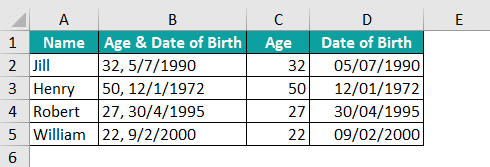
Clearly, we can see that the data in column B is split between columns C and D.
- Using split data in excel, we can organize data effectively.
Table of contents
Key Takeaways
- Split Cells in Excel separates a cell into two or more cells.
- We can split cells in Excel using delimiter, fixed width, and flash fill methods.
- We can also use Excel formulas to split cells. They are:
- RIGHT and LEFT functions provides the specified number of characters from the end and beginning of the text strings, respectively.
- LEN function returns the mentioned number of characters in a text string.
- FIND function gives the location of the substring in a text string.
- #NAME! error occurs when incorrect formulas are entered.
How To Split Cells In Excel Using Text To Columns
We can split cells in excel using two methods. They are:
#1 – Using Delimiter
The Delimiter is a separator that divides the data into different cells. The below example will help us understand the method better. In the table, cell A2 has the full name of a person. So, we need to split the contents of cell A1 between cells B2 and C2 using the Delimiter feature.

The steps to split cells in Excel are as follows:
Step 1: To begin with, we should select the cells which we want to split. So, in this example, let us choose cell A2.
Step 2: Then, select the Text to Columns option from the Data Tools group under the Data tab.
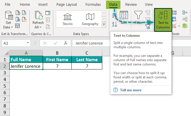
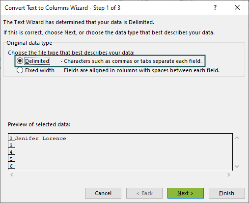
Step 3: First, choose the Delimited radio button in the Convert Text to Columns Wizard – Step 1 of 3 window; click Next>.
Step 4: Next, the Convert Text to Columns Wizard – Step 2 of 3 window appears. Here, check the Space checkbox from the Delimiters list and select Next>.
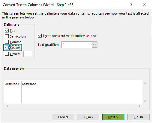
Step 5: At last, select the General radio button from the Column data format list in the window, Convert Text to Columns Wizard – Step 3 of 3.
Finally, in the Destination box, we should set the cell reference where we want to display the result. In this example, the cell reference will be $B$2.
Step 6: Click Finish.

The result is displayed in cells B2 and C2.

Now, the full name ‘Jenifer Lorence’ is split into two cells as ‘Jenifer’ in cell B2 and ‘Lorence’ in cell C2.
- Clearly, we can split data from one cell into multiple cells in excel.
#2 – Using Fixed Width
The Fixed Width splits the excel cells based on the position of the vertical line inserted in the data. Also, it works only when all the substrings have a fixed length.
For example, consider the below table with Date/Time details in column A. So, we need to split the cells’ content into columns B and C using the Fixed Width feature.
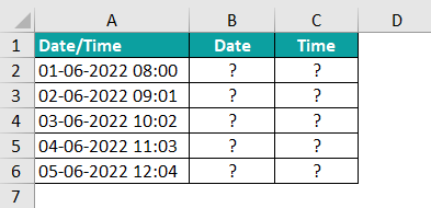
The steps to split cells in excel are as follows:
Step 1: Initially, we need to select the cells which we want to split. In this example, let us choose the cell range A2:A6.
Step 2: After that, choose the Text to Columns option in the Data tab.

Step 3: First, the Convert Text to Columns Wizard – Step 1 of 3 window appears.
Select the Fixed width radio button from the Original data type list and then click Next> to continue.

Step 4: In a few minutes, the second window Convert Text to Columns Wizard – Step 2 of pops up. Click Next>.
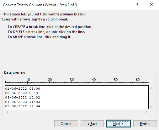
Step 5: Lastly, select the Date radio button in the Convert Text to Columns Wizard – Step 3 of 3 window.
And, in the Destination box, we should set the cell reference where we want to display the result.
So, in this example, the excel cell reference will be $B$2.
Click Finish.

The result is displayed in columns B and C.

We can see that the data in column A is split into two columns, B and C.
For instance, the data, ‘01-06-2022 08:00’ in cell A2 is split into two cells, i.e., ‘01-06-2022’ in cell B2 and ‘08:00’ in cell C2.
- In short, we can use split cells in Excel to divide data into multiple cells.
How To Separate Cells in Excel With Fill Flash?
FLASH FILL in Excel is an automatic data filler. It senses the pattern and automatically fills the data in cells. In addition, it is a very powerful function that reduces user’s time and efforts.
For example, the following table shows the names of fictional characters in column A. So, we need to split the contents of column A into columns B and C using the flash fill function.

The steps to split cells in Excel using the flash fill option are as follows:
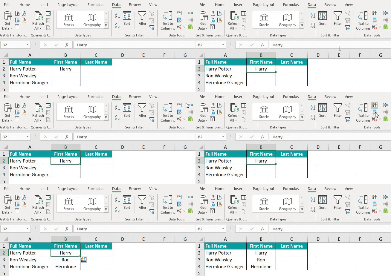
We know that the FLASH FILL function helps to fill the data automatically. So, in this example, let us see how data is flash filled in cells B2 and C2.
Step 1: First, add the table in Excel. Then, type the first name displayed in cell A2, i.e., ‘Harry’ in cell B2.
Step 2: Next, select the Data tab.
Choose the Flash Fill option from the Data Tools group.
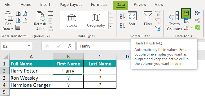
Step 3: The Flash Fill button displays the first name of all the fictional characters in cells B3 and B4.
Likewise, enter the last name, i.e., ‘Potter’ in cell C2.
Step 4: Go to the Data tab.
Step 5: Then, select the Flash Fill option from the Data Tools group.

Clearly, we can see that the Flash Fill button displays the last names of all the fictional characters in cells C3 and C4.
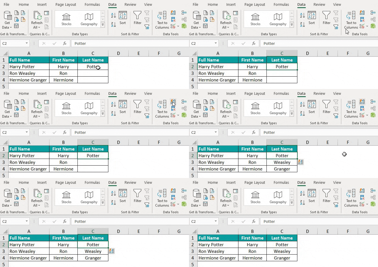
- Therefore, we can split data using flash fill in excel.
How To Divide A Cell With Excel Formulas?
We can use split cells in excel formula to divide a cell.
RIGHT function: The RIGHT function provides the specified number of characters from the end of a text string.
LEFT function: The LEFT function gives the specified number of characters from the beginning of a text string.
LEN function: The LEN excel function returns the mentioned number of characters in a text string.
FIND function: The FIND function gives the location of the substring in a text string.
Divide A Cell With RIGHT, LEFT, LEN and FIND functions
For example, the below table displays the full name, ‘Christopher Columbus’ in cell A2. Let us learn how to split data from A2 to cells B2, and C2 using RIGHT, LEFT, LEN, and FIND functions.

The steps used to divide a cell with excel functions are as follows:
Step 1: We can use RIGHT, LEN, and FIND formulas to split and display the last name, i.e., ‘Columbus’ in cell C2.
So, type the complete formula =RIGHT(A2,LEN(A2)-FIND(” “,A2)) in cell C2.

Step 2: Press Enter to obtain the result.
We can see the last name in cell C2.

- Hence, we can split data from one cell into another using RIGHT, LEN, and FIND functions in excel.
Divide A Cell With LEFT and FIND functions
Similarly, we can use LEFT and FIND formulas to split cells in Excel.
Step 1: First, we need to type the complete formula.
So, type =LEFT(A2,FIND(” “,A2)) in cell B2 to display the first name, i.e., ‘Christopher’ in cell B2.

Step 2: Then, press Enter to obtain the result.
We can see the first name in cell B2.

So, we can split data from one cell into another using LEFT and FIND functions in excel.
Therefore, we can use split cells in Excel formula to divide a cell.
Important Things To Note
- The split cells in Excel feature divide the cell into two or more cells
- Also, it is used to review, filter, sort, and organize lengthy datasets.
- This feature reads commas, spaces, semi colon, and other delimiters in the data to split the cells.
- The shortcut key for the FLASH FILL function is Ctrl + E.
- Using the Split function, we can convert the test series date into data with an actual date.
- We can divide the cells in excel using LEFT, RIGHT, LEN, and FIND formulas.

Frequently Asked Questions (FAQs)
The split cells feature splits a cell’s content into two or more cells. It helps users to organize data with just a click. For example, consider the table below with the list of cities and states in column A. Let us use the following steps to understand how this concept.
The steps to split cells in excel are as follows:
Step 1: To begin with, choose the cell range A2:A4.
Step 2: Then, go to the Data tab.
Step 3: Select Text to Columns option from the Data Tools group.
Step 4: First, the Convert Text to Columns Wizard – Step 1 of 3 window appears.
Select the Delimited radio button and click Next.
Step 5: Next, the Convert Text to Columns Wizard – Step 2 of 3 window appears.
Choose the Comma checkbox and click Next.
Step 6: Lastly, the Convert Text to Columns Wizard – Step 3 of 3 window appears.
Select the General radio button.
Step 7: In the Destination box, enter the cell reference and click Finish.
Finally, we can see that the data in column A is split between columns B and C.
❖Thus, we can organize data using split data in excel.
We can use the split cells in excel shortcut with the below steps:
1. Select the cells which we want to merge.
2. Press Alt + A + E to split cells in excel.
The steps used to split merged cell in Excel are as follows:
Step 1: First, select the Merged cell.
Step 2: Go to Home tab.
Step 3: Then, click the Merge & Center button under the Alignment group.
Step 4: Select the Unmerge Cells option.
Step 5: The cells will be unmerged.
We can also use the split cells in excel shortcut to merge a cell in Excel with the below steps:
● Select the cells which we want to merge.
● Press Alt + H + M + U
We can access split cells in excel feature as shown below:
● Select the cells that we want to merge.
● Select the Data tab.
● Click on the Text to Columns option from the Data Tools group.
Download Template
This article must be helpful to understand Split Cells in Excel, with its formula and examples. You can download the template here to use it instantly.
Recommended Articles
This has been a guide to Split Cells in Excel. Here we discuss how to split cells using delimiter & excel formulas using examples with downloadable template. You can learn more from the following articles –

Leave a Reply