TRUNC in Excel

What is the TRUNC Function in Excel?

The Function TRUNC in Excel returns a numeric value. The “number” argument is the input value that is to be truncated, and the “num_digits” argument is the number of digits after the decimal value. It is also known as the Truncate in Excel. The function is categorized under Excel’s mathematical and trigonometrical functions, introduced in 2007.

For example, we apply the TRUNC function in cell B2 to truncate the value of the given number.

The TRUNC formula is entered in cell B2; the complete formula is =TRUNC(A2), and the result is returned as ‘2.’ Likewise, using TRUNC in Excel function, we can find the output.

What is the TRUNC Function in Excel?

The TRUNC in Excel is also known as the Truncate function in Excel.
The syntax of the TRUNC Excel Formula is =TRUNC(number,[num_digits)] where number is the only mandatory argument.
The function returns numeric value.
If the “num_digits” argument is negative, the value return is zero.
The TRUNC and INT functions are similar functions in Excel because they return the integer part of a number. The difference is that the TRUNC function merely truncates a number, but INT rounds off a number.

TRUNC() Excel Formula

The syntax of the TRUNC in Excel Formula is

number=This is the mandatory argument. This is the number to be truncated.
num_digits=This is the optional argument. This is the number of digits to be truncation. The value given to the “num_digits” argument is as follows:
- If the value is equal to zero, the function will return the rounded value.
- If the value is more than zero, indicate the number of digits to be truncated after the decimal.
- If the value is less than zero, the number of digits must be truncated before the decimal.

Excel VBA – All in One Courses Bundle (35+ Hours of Video Tutorials)

If you want to learn Excel and VBA professionally, then Excel VBA All in One Courses Bundle (35+ hours) is the perfect solution. Whether you’re a beginner or an experienced user, this bundle covers it all – from Basic Excel to Advanced Excel, Macros, Power Query, and VBA.

Start Learning Now

How to Use the TRUNC Excel Function?

We can insert TRUNC in excel using the below two methods

1. Access from the Excel ribbon

First, choose the empty cell which will contain the result.
Next, go to the Formulas tab.
Then, select the Math & Trig option from the drop-down menu.
Also, select TRUNC from the menu.
A window called Function Arguments appears.
As the number of arguments, enter the value in the “number” & “num_digits.”
Select OK.

2. Enter the worksheet manually

Select an empty cell for the output.
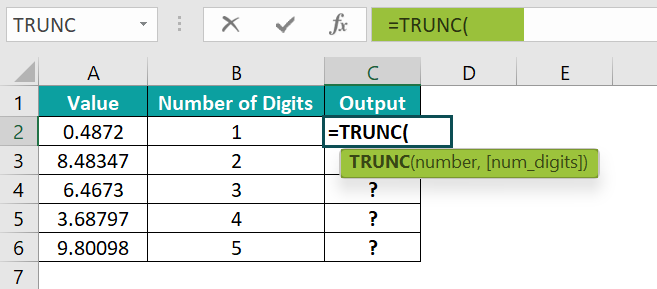
Type =TRUNC( in the selected cell. Alternatively, type =T and double-click the TRUNC function from the list of suggestions shown by Excel.
Press the Enter key.

Let us take an example to understand this function in detail. The succeeding example depicts the numbers, and now, we will truncate the unwanted digits using the Excel TRUNC function.

In the table, the data is reflected as below: –

Column A contains the Value.
Column B contains the Number of Digits.
Column C contains the Output.

The steps to evaluate the values by the Function TRUNC in Excel are as follows:

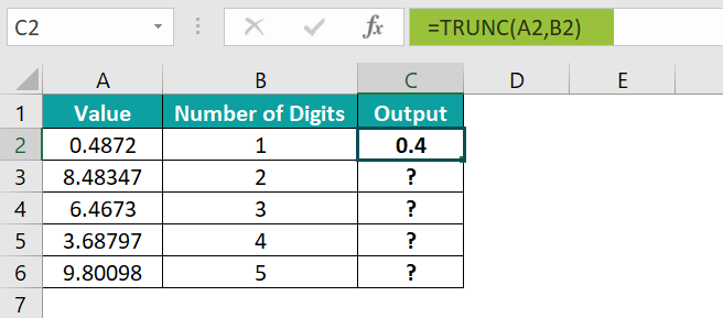
First, select the cell where we will enter the formula and calculate the result. The selected cell, in this case, is cell C2.
Next, we will enter the TRUNC in the Excel formula in cell C2.
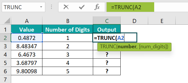
Then, enter the value of ‘number’ as A2, i.e., the value we need to truncate.
Next, enter the value of ‘num_digits’ as B2, i.e., the number of digits we want to truncate.
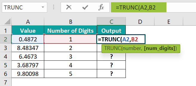
So, the complete formula is =TRUNC(A2,B2) in cell C2.
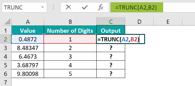
Next, press the “Enter” key. The results in cell C2 are “0.4” in the image below.
Press enter and drag the cursor to cell C6, as shown in the following image.

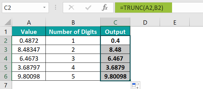
Likewise, using TRUNC in excel function, we can find the output.

Examples

Example #1

The succeeding example depicts the Date and Time as values, and now, we will truncate the Time using the Date TRUNC in the Excel function.

In the table,

Column A contains the Date & Time.
Column B contains the Number of Digits.
Column C contains the Output.

The steps to evaluate the values by the Function TRUNC in Excel are as follows:

Step 1: First, select the cell where we will enter the formula and calculate the result. The selected cell, in this case, is cell C2.

Step 2: Next, we will enter the TRUNC Formula in the Excel in cell C2.

Step 3: Then, enter the value of ‘number’ as A2, i.e., the value we need to truncate.

Step 4: Also, enter the value of ‘num_digits’ as B2, i.e., the number of digits we want to truncate.

Step 5: The complete formula is =TRUNC(A2,B2) in cell C2.

Step 6: After entering each value in the preceding step, press the “Enter” key. The results in cell C2 are “02-01-2000” in the image below.

TRUNC Function in Excel - Example 1 - Step 6.gif

Step 7: Next, press enter and drag the cursor to cell C6, as shown in the following image.

TRUNC Function in Excel - Example 1 - Step 7

Likewise, we can use TRUNC function to find values.

Example #2

The succeeding example depicts the Date and Time as values, and we will truncate the Date using the Excel TRUNC function.

In the table,

Column A contains the Value.
Column B contains the Number of Digits.
Column C contains the Output.

The steps to evaluate the values by the Function TRUNC in Excel are as follows:

Step 1: To begin with, select the cell where we will enter the formula and calculate the result. The selected cell, in this case, is cell C2.

Step 2: Next, we will enter the TRUNC Excel formula in cell C2.

Step 3: Then, enter the value of ‘number’ as A2, i.e., the value we need to truncate.

Step 4: Also, enter the value of ‘num_digits’ as B2, i.e., the number of digits we want to truncate.

Step 5: So, the complete formula is =TRUNC(A2,B2) in cell C2.

Step 6: After entering each value in the preceding step, press the “Enter” key. The results in cell C2 are “05:02:24” in the image below.

Step 7: Press enter and drag the cursor to cell C6, as shown in the following image.

Likewise, using TRUNC function, we can find the output.

Example #3

The succeeding example depicts the Negative numbers, and we will truncate the unwanted digits using the Excel TRUNC function.

In the table,

Column A contains the Value.
Column B contains the Number of Digits.
Column C contains the Output.

The steps to evaluate the values by the Function TRUNC in Excel are as follows:

Step 1: First, select the cell where we will enter the formula and calculate the result. The selected cell, in this case, is cell C2.

Step 2: Next, we will enter the TRUNC Excel formula in cell C2.

Step 3: Then, enter the value of ‘number’ as A2, i.e., the value we need to truncate.

Step 4: Likewise, enter the value of ‘num_digits’ as B2, i.e., the number of digits we want to truncate.

Step 5: So, the complete formula is =TRUNC(A2,B2) in cell C2.

Step 6: After entering each value in the preceding step, press the “Enter” key. The results in cell C2 are “-2” in the image below.

Step 7: Press enter and drag the cursor to cell C6, as shown in the following image.

Similarly, we can use TRUNC function to obtain values.

Important Things to Note

The TRUNC function is categorized under the Math & Trig functions in the Function Library.
The function returns a negative value less than zero, specifying the number of digits to the left of the decimal point.
The TRUNC formula returns equal to zero, which specifies the rounded value to the nearest integer.
The TRUNC excel function returns a positive value greater than zero, specifying the number of digits to the right of the decimal point.

Frequently Asked Questions (FAQs)

1. What does the TRUNC function do in Excel?

The TRUNC Function in Excel truncates a number to the prescribed number of decimal places. The function can also truncate a number to a given precision. It also extracts dates from date and time values.

The TRUNC function is a built-in function in Excel that is categorized as a Math & Trig Function in Excel. The function was introduced in MS Excel in 2007.

The syntax of the TRUNC function is as follows;
=TRUNC(number,[num_digits])

2. How does the TRUNC function work in Excel?

The TRUNC function works in Excel by following the below steps;
• First, select an empty cell for the output.
• Next, type =TRUNC( in the selected cell. Alternatively, type =T and double-click the TRUNC function from the list of suggestions shown by Excel.
• Then, press the “Enter” key.

For example, we apply the TRUNC function in cell B2 to truncate the value of the given number.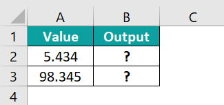

The TRUNC formula is entered in cell B2; the complete formula is =TRUNC(A2), and the result is returned as ‘5 & 98.’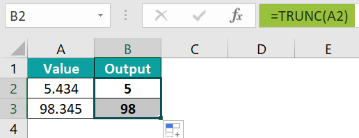

3. Where is the TRUNC Function in Excel?

We can insert TRUNC in Excel using the following steps:
• First, choose the empty cell which will contain the result.
• Next, go to the Formulas tab.
• Then, select the Math & Trig option from the drop-down menu.
• Also, select TRUNC from the menu.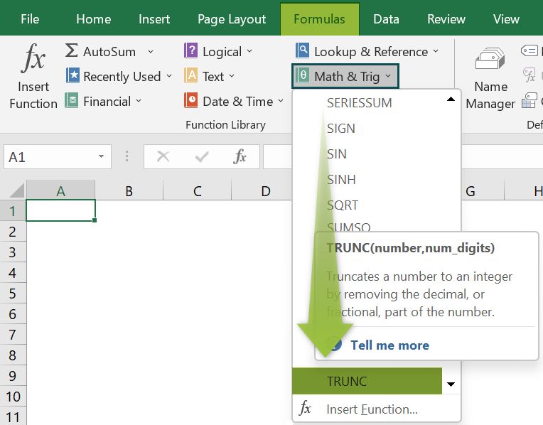

• A window called Function Arguments appears.
• As the number of arguments, enter the value in the “number” & “num_digits.”
• Select OK.

Download Template

This article must help understand the TRUNC Excel Function’s formula and examples. You can download the template here to use it instantly.

TRUNC in Excel Download

TRUNC in Excel