
What Is VALUE Function In Google Sheets?
The VALUE function in Google Sheets is a built-in Text function. It accepts a text string and determines the number the text string represents.
Users can make use of the VALUE() in Google Sheets to convert texts to numbers, extract number values from the specified texts, and validate the user-fed data. The function also helps sanitize data imported into a Google Sheets file.
Use this VALUE Function In Google Sheets Template to follow along with the examples in this article.
Download Excel TemplateFor instance, we have a set of input values in column A.

The requirement is to determine the numbers the listed values represent and showcase the output in column B.
Then, we can apply the VALUE() in the target cells to fetch the output, in line with the meaning of the VALUE function in Google Sheets explained earlier.

The VALUE() accepts one input value, similar to the Excel VALUE function.
When the supplied argument value is a number in a Google Sheets-recognized number format, the VALUE function in Google Sheets returns the number. However, the output will be in the number format Google Sheets considers at the backend for evaluation.
In the case of the cell B2 formula, the VALUE function in Google Sheets argument is a number value of 35%. So, the function output is 0.35, the same number in its raw form.
On the other hand, when the supplied input value to the VALUE() is a date-time value, the function returns the serial number equivalent of the date-time value as in cell B3. While the whole part is the serial number equivalent to the date, the decimal part indicates the time value.
However, if the provided VALUE function in Google Sheets argument is a text value, the function returns the #VALUE! error value. The reason is that the input value does not translate into a number value.
Furthermore, if the supplied input argument is a currency value, the VALUE function in Google Sheets returns the currency value as a number without any currency formatting.
Key Takeaways
- The VALUE function in Google Sheetstakes one value as the input to evaluate the number the cited value translated into or represents.
- The VALUE formula in Google Sheets is helpful while performing data validation, translating text values into numbers, and pulling number values from the given texts.
- The VALUE formula in Google Sheets accepts one mandatory argument, text,as the input.
- We can apply the VALUE formula in Google Sheets as a standalone function. However, using the function with other inbuilt functions, such as IF, RIGHT, and LEN,makes it highly productive.
VALUE() Google Sheets Formula
The VALUE formula in Google Sheets syntax is the following:

Where,
- text: The text containing the value we aim to convert into a number value.
Please ensure to supply the argument value when using VALUE function in Google Sheets.
How To Use VALUE Function In Google Sheets?
We can utilize the function VALUE in Google Sheets in the following ways:
- Access the function from the ribbon.
- Enter the function into the sheet manually.
Method #1 – Access The Function From The Ribbon
Select a target cell for displaying the result → The Insert tab → The Function option right arrow → The Text function group right arrow → The VALUE function.

The chosen function appears in the target cell, with the cursor within the function brackets. We can now enter the function argument within the brackets.

Further, click the ‘?’ symbol against the function name to know the function syntax.

We can then click the down arrow in the syntax window to know the meaning of the VALUE function In Google Sheets explained with the help of a basic example.

Finally, press Enter to acquire the function output.
Method #2 – Enter The Function Into The Sheet Manually
- Select the target cell where we aim to showcase the result.
- Type =VALUE( in the cell.
[ Alternatively, type =V or =VA and click the function name VALUE from the listed options to choose the function.]
- Enter the argument value and close the brackets.
- Press Enter to fetch the VALUE function output in Google Sheets.
Examples
The examples below show the practical ways of using VALUE function in Google Sheets.
Example #1
The source dataset lists employees and their swipe-in and out times.

We must find the total working hours each employee clocked and show the output in column D.
- Step 1: Select cell D2, enter the VALUE(), and press Enter.
=VALUE(C2)-VALUE(B2)

[ Alternatively, select the target cell and then Insert → Function → Text → VALUE function.

The chosen function will appear in the target cell.

Complete the required formula in the target cell.


Finally, press Enter to view the value the formula returns.]
- Step 2: Utilize the fill handle to update the formula in the remaining target cells.

The VALUE() output in each target cell is a decimal value, which we might find challenging to interpret as the total working hours clocked value. So, select the target cells D2:D6, click the More formats option, and then the applicable time format.

Thus, now we can view the output in a time format, which is more understandable. For instance, the total working hours clocked by the first employee is 10 hours (Between 8:30 AM to 6:30 PM).

Example #2
The following dataset shows the description of the monthly inventory level data at a firm.

We must show only the monthly inventory level value in column C cells based on the corresponding descriptions. After that, the requirement is to update the total inventory level in cell C9, considering the determined column C inventory level values.
- Step 1: Choose cell C2, enter the VALUE() containing the RIGHT() and LEN(), and press Enter.
=VALUE(RIGHT(B2,LEN(B2)-24))

First, the LEN(), which works like the Excel LEN function, finds the total count of characters in cell B2, which is 26. Next, the formula deducts 24 from 26, which results in a value of 2. Next, the RIGHT(), with the logic similar to Excel RIGHT function, accepts the cell B2 text and counts two characters from the right end of the input value, which is the number 25.
Finally, the VALUE() accepts the RIGHT() output value of 25 as the input. Since the input value is a number, the function returns the number as is, 25.
Next, the input text length and the required number length are the same in all the cells B2:B7. So, we can apply the same formula in all the required cells.
- Step 2: Use the fill handle to feed in the formula in cells C3:C7.

Thus, we have the numbers extracted from the texts using the VALUE().
- Step 3: Choose cell C9, enter the SUM(), and press Enter.
=SUM(C2:C7)

The SUM(), which works like the Excel SUM function, takes the numbers cited in cells C2:C7 as the input to return 111 as the required total inventory level.
Example #3
Consider the task deadline at a firm is 7 PM.
We have a list of tasks and their finish times in columns A and B. Next, we find the difference between the actual finish time and the deadline for each task to determine the delay in the respective task completion, with the values being in minutes. This data is cited in column C.

We must determine the penalty points for each task based on the delay in completing the corresponding task, with the points increasing by 2 points with a higher delay. Assume the target cells are D4:D8.
- Step 1: Choose cell D4, enter the IF() containing the VALUE(), and press Enter.
=IF(C4=VALUE(“0:00”),0,IF(C4<VALUE(“0:05”),2,IF(C4<VALUE(“0:10”),4,IF(C4<VALUE(“0:15”),6,IF(C4<VALUE(“0:20”),8,10)))))

- Step 2: Use the fill handle to implement the formula in the remaining target cells.

Let us see the cell D8 formula to know how it works.
First, the VALUE() in the outer-most IF() condition accepts the minute value of 0:00 as input to return 0 as the number the input value represents. The IF(), which has the same logic as the Excel IF function, checks if the cell C8 value equals 0. Since the decimal equivalent of 0:18 is 0.0125, the condition is false. So, the IF() in the FALSE value executes.
The VALUE() in this IF() condition returns the number the minute value of 0:05 represents, 0.003472. The IF() checks if the cell C8 value of 0.0125 is below 0.003472. Since the condition is false again, the IF() in the FALSE value executes.
Next, the VALUE() in this IF() condition returns the number the minute value of 0:10 represents, 0.00694. The IF() checks if the cell C8 value of 0.0125 is below 0.00694. Since the condition is false again, the IF() in the FALSE value executes.
Next, the VALUE() in this IF() condition returns the number the minute value of 0:15 represents, 0.01041. The IF() checks if the cell C8 value of 0.0125 is below 0.01041. Since the condition is false again, the IF() in the FALSE value executes.
Next, the VALUE() in this IF() condition returns the number the minute value of 0:20 represents, 0.01388. The IF() checks if the cell C8 value of 0.0125 is below 0.01388. The IF() condition is true. So, the function returns the TRUE value, 8, as the required penalty points for the concerned task.
VALUE Function Returns #VALUE Error
The VALUE function returns the #VALUE! error in Google Sheets in the following scenarios:
- The supplied argument value is non-numerical and does not translate into a number value.
- The supplied argument value is not in a Google Sheets-recognized number format.
Important Things To Note
- When the supplied text argument value is an empty text string or a reference to an empty cell, the output of the VALUE function in Google Sheetsis 0.
- The supplied text argument value can be in a Google Sheets-recognized constant number, date, or time format. However, when the text argument value is not in any of these formats, the Google Sheets VALUE function returns the #VALUE! error value.
- Typically, we do not need to include the VALUE() in an expression because Google Sheets automatically changes text values to numbers according to the requirement. So, the function is available in Google Sheets for compatibility with other spreadsheet applications.
Frequently Asked Questions (FAQs)
We can use the VALUE function with Data Validation in Google Sheets, as explained below with an example.
The source dataset lists dates in column A and we must update the daily sales data in the corresponding column B cells.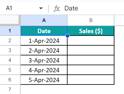
However, assume we enter a value in a cell, which is not a number or it is a value not in the Google Sheets-recognized number format. Then, we must see an error warning message against the cell, so that we can update the correct value in the right number format in the specific cell.
Then, we can use a VALUE function-based custom formula in the Data Validation feature in Google Sheets to achieve the required outcome.
• Step 1: Select the range B2:B6 and then Data → Data validation.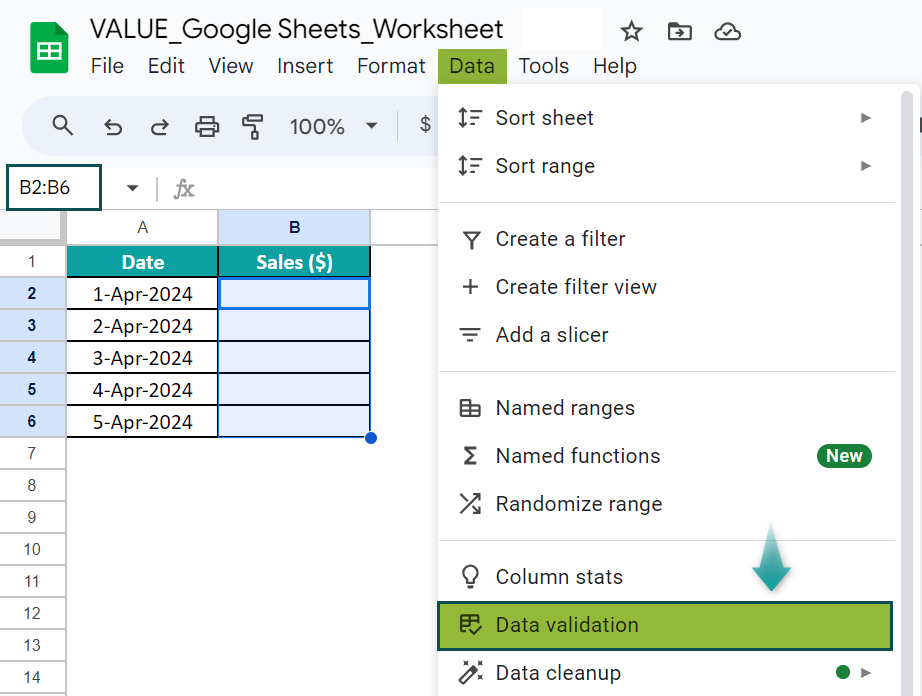
• Step 2: The Data validation rules pane will appear on the right of the work area, where we must click the + Add rule option.
• Step 3: The Apply to range field shows the chosen range.
Next, click the Criteria field dropdown button to set the field as the Custom formula is option. After that, enter the VALUE function-based custom formula.
=IFERROR(VALUE(B2),””)
Next, update the applicable Advanced options fields.
Finally, click Done and close the Data validation rules pane.
Now, enter the required sales data in the valid currency format, as shown below.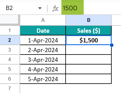
Assume we enter the word “Thousand” instead of the value $1,000 in one of the target cells.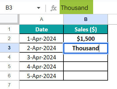
However, when we press Enter, we will see the error message.
Thus, we can immediately update the correct value in the concerned cell.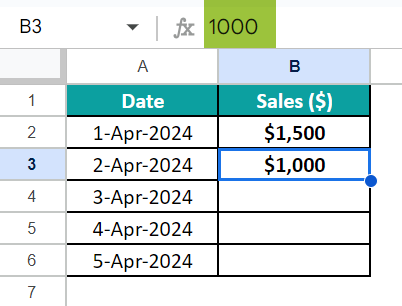
Likewise, we can update the required sales data as valid numbers in the appropriate number format in the remaining target cells.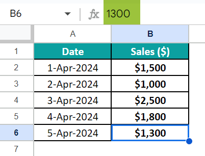
The VALUE function in Google Sheets is not working because of the following reasons:
• The function name is incorrect.
• The supplied text argument value is non-numerical.
• The provided text argument value is numeric but not in a Google Sheets-recognized number format.
We can convert text to numbers in Google Sheets apart from using the VALUE function using the following techniques:
• Use the number formatting options from the ribbon or the Format tab.
• Use the REGEXREPLACE function.
Use this VALUE Function In Google Sheets Template to follow along with the examples in this article.
Download Excel Template