Format Number In VBA Excel
Formatting is a common task when we prepare reports in Excel. Formatting the numbers is very important to make the user understand the numbers quickly with formatting. In VBA, we can apply the number formatting by using several methods, such as the FORMAT function, the FORMAT NUMBER function, and the NUMBER FORMAT property.
For example, assume we have the number 0.90 i.e., 90%, and if we want to apply the percentage format for this number, then, we can use the FORMAT like the following.
FORMAT(0.90, “Percent”)
This will format the number and returns the number in percentage i.e., 90%.
Key Takeaways
- The number Formatting property helps us to apply the desired formatting to a given range of cells.
- We can apply different number formatting like percentage, currency, date, time, etc.
- We can apply colored number formatting based on the various criteria within the number formatting code.
- We can opt to show only the date or time when we have both the date and time.
- We can show the text along with the numbers by formatting numbers with the text.
Excel VBA 5-in-1 Course Bundle – (30+ Hours of Expert-Led Training)
If you want to learn Excel and VBA professionally, then the Excel VBA 5-in-1 Course Bundle (30+ hours) is the perfect solution. Whether you’re a beginner or an experienced user, this bundle covers it all – from Basic Excel VBA to Event Automation, Error Handling, Email Automation, and real-world applications with downloadable templates.
How To Format Numbers With VBA Number Format?
Number Format is the property available with the range of cells in VBA. For example, look at the following numbers.
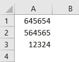
In a range of cells A1:A3, we have the numbers. If we want to apply number formatting for these numbers, then we can utilize the number format property.
Step 1 – Before we apply the number formatting, we need to identify the range of cells where we need to apply the number formatting i.e., A1:A3.
Enter the desired range of cells using the RANGE object like the following.
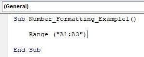
Step 2 – Once the number formatting is given, enter the dot to access the IntelliSense list, which shows all the properties and methods available with the RANGE object.
Enter the dot and start typing the property name NumberFormat and we will see the IntelliSense list showing the list.

Choose the Number Format property from the list.
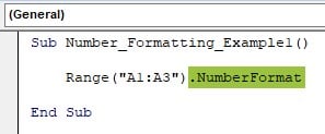
To apply the number format, we need to be ready with the number format code. We will learn some of the ready codes. As of now, apply the formatting code “#,##,###” by entering an equal sign after the number format property.

This will apply the custom number formatting with thousand separators like the following.
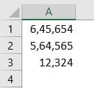
Likewise, by entering the number formatting code, we can apply the formatting. Following are some examples of applying the number formatting.
GENERAL
Range(“A1:A3”).NumberFormat = “General”
Number
Range(“A1:A3”).NumberFormat = “0.00”
Currency
Range(“A1:A3”).NumberFormat = “$#,##0.00”
Accounting
Range(“A1:A3”).NumberFormat = “_($* #,##0.00_);_($* (#,##0.00);_($* “”-“”??_);_(@_)”
Percentage
Range(“A1:A3”).NumberFormat = “0.00%”
Fraction
Range(“A1:A3”).NumberFormat = “# ?/?”
Scientific
Range(“A1:A3”).NumberFormat = “0.00E+00”
Text
Range(“A1:A3”).NumberFormat = “@”
Apart from these number formatting, we can also apply custom formatting. Let us discuss the same in detail now.
Examples
Example #1 – Differentiation Between Positive And Negative Numbers
It is quite common that we will be having both positive and negative numbers in our reports. To make the users understand things quickly, we can apply different number formatting for positive and negative numbers. For example, look at the following data in Excel.
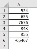
We have numbers from cells A1 to A6. This list contains both positive numbers and negative numbers.
Our aim is to apply the number formatting that shows all the negative numbers in red. Let’s apply this formatting.
Step 1: To get access to the number format property, first, provide the range of cells by using the RANGE object.
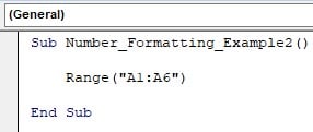
Step 2: By entering the dot, choose the number format property.

Step 3: Apply the following number formatting code.
“#,##.00;[red]-#,##.00”

Step 4: Once we run this code, it will apply the number formatting and also makes the negative values red color.

Step 5: As we can see, all the negative numbers are in red color. The number formatting code that we have applied also includes the decimal places, if we don’t want to show the decimal places, then remove the zeros from the code as follows.
“#,##;[red]-#,##”

Code with Decimal Place
Sub Number_Formatting_Example2()
Range(“A1:A6”).NumberFormat = “#,##.00;[red]-#,##.00” .
End Sub
Code without Decimal Place
Sub Number_Formatting_Example2()
Range(“A1:A6”).NumberFormat = “#,##;[red]-#,##”
End Sub
Example #2 – Show Negative Values In Brackets
It is a common practice to show the negative numbers in brackets. To show the negative numbers in the bracket, we need to include parenthesis for the negative portion of the formatting code.
“#,##;[red](-#,##)”
As we can see, above the yellow-colored code, there is a parenthesis.
Sub Number_Formatting_Example3()
Range(“A1:A6”).NumberFormat = “#,##;[red](-#,##)”
End Sub
This will include the parenthesis for all the negative numbers.

Example #3 – Text With Numbers
This is an interesting example. Assume we have numbers to show but not in regular number formatting along with the text.
For example, if we are showing the numbers of vegetable weight, we have to show it in KGS i.e., 10 KG or 5 TONS.
We can show numbers as well as text by applying the formatting. For instance, look at the following data.

We have a person’s name and their respective weight. We must apply the formatting for this weight column as KG after the weight number.
The following code will format the number along with the text “KG”.
“0#”” KG”””
Sub Number_Formatting_Example4()
Range(“B2:B6”).NumberFormat = “0#”” KG”””
End Sub
This will include the text KG after every number in the range B2 to B6.

Similarly, if we want to include any other text, we can simply replace the KG with any other words.
Example #4 – Apply Conditional Number Formatting
Applying formatting for numbers based on the condition is another important formatting technique we need to be aware of.
For example, look at the following data.

We have student names and their respective scores in an examination. Now we need to apply the number formatting that shows all the numbers greater than or equal to 50 in Green and all the numbers less than 50 in Red.
The following number formatting code will apply Green font formatting for values greater than or equal to 50 in Green and all the numbers less than 50 in Red.
“[>=50][Green]#,##0.00;[<50][Red]#,##0.00”
Sub Number_Formatting_Example5()
Range(“B2:B9”).NumberFormat = “[>=50][Green]#,##0.00;[<50][Red]#,##0.00”
End Sub
The number formatting looks like the following image.

Example #5 – Apply Date And Time Format
By using the number format property, we can apply the date and time format as well. For example, look at the following date.

Let us apply various date and time formats.
Date -Month-Year format
Sub Number_Formatting_Example6()
Range(“A2”).NumberFormat = “dd-mm-yyyy”
End Sub
This will apply the date format like the following image.

Date and Time Format
Sub Number_Formatting_Example6()
Range(“A2”).NumberFormat = “dd-mm-yyyy hh:mm:ss”
End Sub
This will apply the date and time format as shown in the following image.

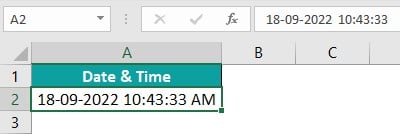
To show the time in AM or PM, use the following code.
Sub Number_Formatting_Example6()
Range(“A2”).NumberFormat = “dd-mm-yyyy hh:mm:ss AM/PM”
End Sub
This will show AM or PM, as highlighted in the below image.
Important Things To Note
- Number Format is a property available with a range of cells. We need to use either the RANGE object or the CELLS property.
- We must be sure of the formatting code to apply the correct number formatting. It is advised to practice the codes in worksheet formatting and then implement the same in VBA coding.
- To show text along with the numbers, we need to include the text in double quotes within the number formatting.
- We need to use an equal sign after the number format property to apply the desired number formatting.

Frequently Asked Questions (FAQs)
The number format in Excel is available under the Home tab.
We can also access the number format window by using the shortcut keys Ctrl + 1 by selecting the desired cell.
To change the number format in VBA, we need to first provide the range of cells, where we need to apply the number formatting like the following.
Then enter the dot and choose the NumberFormat property.![]()
After accessing the number format property, enter an equal sign and enter the desired number format code in double quotes.![]()
To change the text to number format, we need to use the following code.
When the number is stored as text, we cannot number formatting to those cells. First, we need to change the cell to number format and then apply the number formatting.
Another reason could be because of the wrong formatting code given to the number format property. We need to use the appropriate number formatting code to make it work.
Download Template
This article must be helpful to understand the VBA Format Number, with its formula and examples. You can download the template here to use it instantly.
Recommended Articles
This has been a guide to VBA Format Number. Here we explain How To Format Numbers With VBA code and downloadable excel template. You may learn more from the following articles –

Leave a Reply